Tutorial 4: Multiple Testing
February 3, 2026
The Multiple Testing Problem & Adjustment ProceduresCRITICAL: Regular practice with R and RStudio, the statistical software used in BIOL 322 and introduced during tutorial sessions, and consistent engagement with tutorial exercises are essential for developing strong skills in Biostatistics.
EXERCISES: Tutorial reports are independent exercises and are not submitted for grading; however, students are strongly encouraged to complete them. Some tutorials include solutions at the end to support self-assessment and review. Other tutorials do not require model answers because they are procedural and can be easily self-assessed by verifying that the code runs correctly and produces the expected type of output.
General setup for the tutorial
A good way to work through is to have the tutorial opened in our WebBook and RStudio opened beside each other.
*NOTE: Tutorials are produced in such a way that you should be able to easily adapt the commands to your own data! And that’s the way that a lot of practitioners of statistics use R!
Understanding the issues of inflated Type I error when conducting multiple tests
Consider a one-way ANOVA with 10 groups (treatments) in which the null hypothesis H0is true; namely, all groups come from populations with the same mean. Let the population mean be 10 and the population standard deviation be 3. We randomly sample observations from this population and assign them to 10 groups of 7 observations each. Any differences among group means therefore arise solely from sampling variation. We can then run a one-way ANOVA on this simulated dataset:
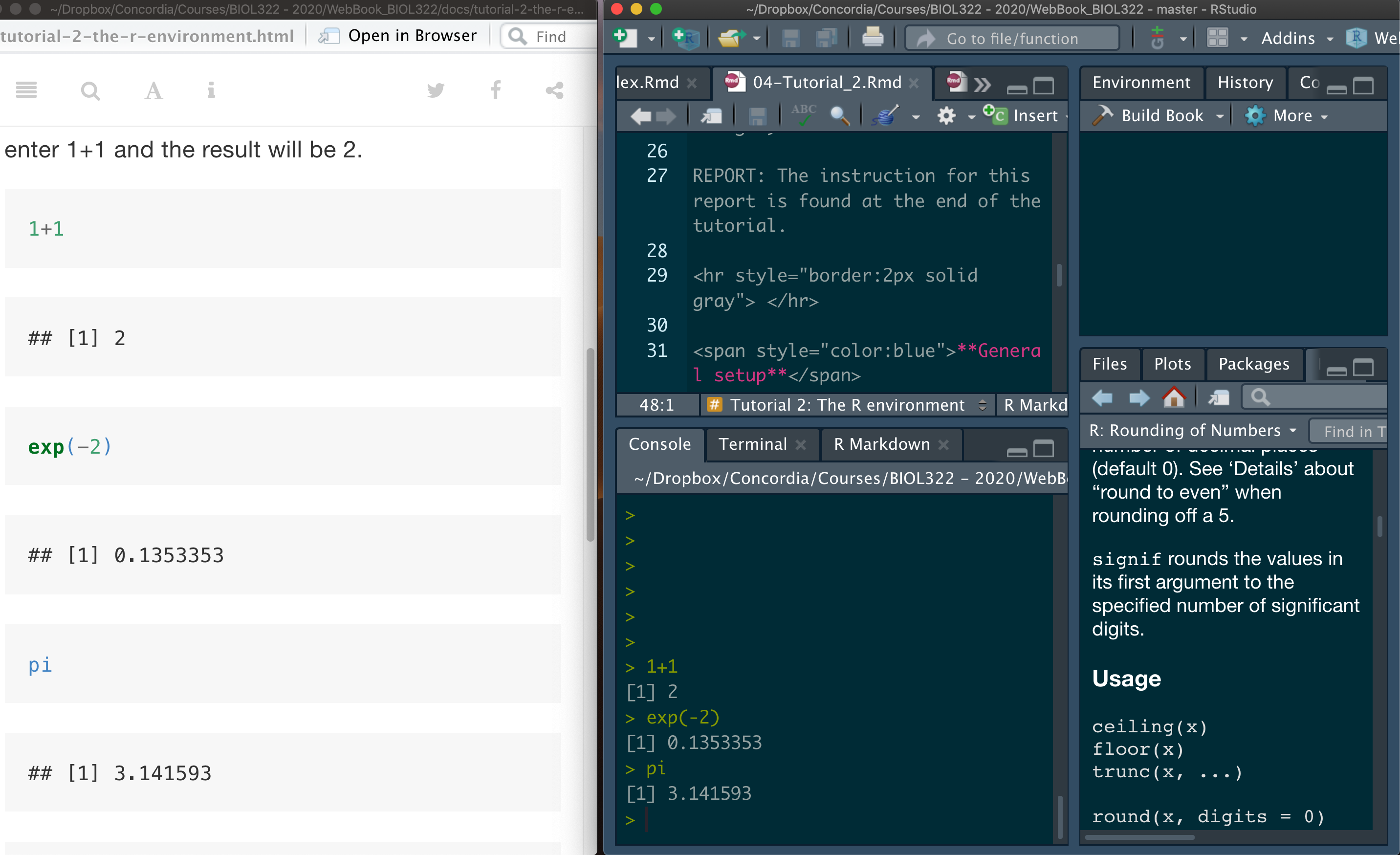
Data.simul <- matrix(rnorm(70,mean=10,sd=3))
View(Data.simul)
Groups <- rep(1:10,each=7)
View(as.matrix(Groups))
Let’s run an ANOVA on the simulated data and extract the P-value from the ANOVA table:
result.lm <- lm(Data.simul~Groups)
anova(result.lm)
anova(result.lm)$"Pr(>F)"[1]
As expected, because all samples were drawn from the same population, the null hypothesis is unlikely to be rejected at a significance level of alpha = 0.05; in other words, the ANOVA should (for this simulated example) typically yields a P-value greater than alpha. However, “unlikely” does not mean “never.” Remember that in frequentist statistical hypothesis testing, we assume that decisions are made under uncertainty and that the significance level alpha represents a long-run error rate. Even when the null hypothesis H0 is true, we still expect it to be rejected by chance alone in a proportion alpha repeated analyses (or repeated realizations of the data-generating process). In this case, that means we should observe false rejections (Type I errors or false positives) in about 5% of repeated ANOVAs, simply due to random sampling variation and the way the statistical testing procedure is set (i.e., to reject alpha% of sample tests even if they are wrong, i.e., false positives).
To see this explicitly, we now repeat the sampling process many times and record how often the null hypothesis H0 is rejected; that is, how often the ANOVA P-value falls below alpha when the null hypothesis is true. This allows us to understand that the rate of false positives (Type I errors) under H00 is alpha. To do this efficiently, we again use the functions lapply and sapply to repeat the same analysis across many simulated datasets. Here, we generate and analyze 1,000 datasets drawn from the same population described above.
This will take about a minute or so to run depending on the computer:
n.tests <- 10000
data.simul <- data.frame(replicate(n.tests,rnorm(n=70, mean=10, sd=3)))
lm.results <- lapply(data.simul, function(x) {
  lm(x~as.factor(Groups), data = data.simul)
})
ANOVA.results <- lapply(lm.results, anova)
P.values <- sapply(ANOVA.results, function(x) {x$"Pr(>F)"[1]})
TypeIerror <- length(which(P.values<=0.05))/n.tests
TypeIerror
Pretty close to alpha = 0.05, right? With a finite number of simulations, we expect some random deviation around this value. If the simulation were repeated an infinite number of times, the proportion stored in TypeIerror (i.e., the false-positive rate) would be exactly to 0.05; meaning that 5% of tests would reject H0 even when H0 is true.
The issue here is that we ended up with about 500 (0.05 * 10000) tests that were significant when the null hypothesis H0 was true. Let’s use the Bonferroni and the FDR adjustments for multiple tests to adjusted these p-values:
p.bonf <- p.adjust(P.values,method="bonferroni")
p.fdr<- p.adjust(P.values,method="fdr")
Let’s view the original and the adjusted p-values:
View(cbind(P.values,p.bonf,p.fdr))f you inspect the adjusted P-values, you will see that none of them are considered statistically significant after correction; even though about 500 of the original (unadjusted) P-values were below . We can also verify this explicitly by counting the number of significant results before and after adjustment, as shown below:
length(which(p.bonf <= 0.05))
length(which(p.fdr <= 0.05))
In real applications, results typically include a mixture of true positives and true negatives, along with some false positives and false negatives. Multiple-testing adjustments to P-values are designed to balance these outcomes by controlling error rates. This trade-off represents the ability to reduce the risk of Type I errors (false positives) while attempting to limit the loss of power that leads to Type II errors (false negatives). Different adjustment methods represent different compromises along this trade-off, depending on how strongly we want to guard against false discoveries.
Multiple-Testing Corrections for Post-Hoc Comparisons in One-Factor ANOVA
Let’s use the “The knees who say night” data from Whitlock and Schluter (2009) as used in tutorial 3; The Analysis of Biological Data.
Let’s load the data:
circadian <- read.csv("chap15e1KneesWhoSayNight.csv")From Tutorial 3, we know that the variances of the three groups (treatments) do not differ significantly, so the homogeneity of variance assumption for ANOVA is satisfied. We also found that the one-way ANOVA was statistically significant, indicating that at least two group means differ. The natural next question is: which groups differ from each other?
To answer this, we conduct pairwise comparisons between group means using t-tests. Because multiple comparisons are involved, P-value adjustments are required. In the code below, we illustrate three cases: no adjustment, the Bonferroni correction, and the False Discovery Rate (FDR) procedure. The FDR method is specified as “BH”, after its original authors, Benjamini and Hochberg. In the function, g simply identifies the grouping variable (the treatment factor).
pairwise.t.test(circadian$shift, g = circadian$treatment,p.adjust.method="none")
pairwise.t.test(circadian$shift, g = circadian$treatment,p.adjust.method="bonferroni")
pairwise.t.test(circadian$shift, g = circadian$treatment,p.adjust.method="BH")
Without any correction for multiple testing, two pairwise comparisons are statistically significant: control vs. eyes (P = 0.0029) and eyes vs. knee (P = 0.0044). In contrast, the comparison between control and knee is not significant (P = 0.9418). These results suggest that the eyes treatment differs from both the control and knee treatments, while control and knee do not differ from each other.
After applying the Bonferroni correction, which is highly conservative, the same pattern of differences is retained, but P-values increase due to the adjustment. Both control vs. eyes (adjusted P = 0.0088) and eyes vs. knee (adjusted P = 0.0132) remain statistically significant, whereas control vs. knee remains clearly non-significant (adjusted P = 1.0000).
Using the False Discovery Rate (FDR) procedure (Benjamini–Hochberg), the results again support the same biological conclusion. The comparisons control vs. eyes (adjusted P = 0.0066) and eyes vs. knee (adjusted P = 0.0066) remain significant, while control vs. knee remains non-significant (adjusted P = 0.9418). Compared to Bonferroni, the FDR adjustment is less conservative, leading to smaller adjusted P-values while still controlling false discoveries.
Importantly, although the numerical P-values differ across methods, all three approaches lead to the same inferential conclusion: the eyes treatment differs from both control and knee, whereas control and knee do not differ from each other.
Note that this function returns adjusted P-values for pairwise (i.e., two-at-a-time) comparisons of group means. In practice, these results are best reported in a summary table that includes, for each contrast, the observed t-statistic, the original (uncorrected) P-value, and the corrected P-value (as illustrated in the lecture). To the best of my knowledge, there is no single standard R function that produces such a comprehensive table directly. For this reason, I wrote two dedicated functions—provided in this tutorial—that generate these tables for one-way and two-way ANOVA designs.
Download the pairwise t table functions
The two functions are included the file (pairwise.t.table.R) and can be loaded into R using the command source as follows:
source("pairwise.t.table.R")There are two functions in the file pairwise.t.table. If you want to look into the code of each function, you can simply type their names:
pairwise.t.table.oneWay
pairwise.t.table.twoWay
For the FDR correction (BH stands for “Benjamini and Hochberg”, the authors of the procedure)
pairwise.t.table.oneWay(circadian$shift,g=circadian$treatment,method="BH")For the Bonferroni correction:
pairwise.t.table.oneWay(circadian$shift,g=circadian$treatment,method="bonferroni")As expected, the adjusted P-values (AdjP) are always larger than the unadjusted P-values (unAdjP), because correction procedures account for the inflation of false positives caused by multiple testing. In practice, we typically report results using a single correction method rather than presenting multiple adjusted P-values. Although the choice depends on the scientific context, I generally recommend the False Discovery Rate (FDR) approach in most cases, as it offers a better balance between controlling false positives and retaining statistical power than more conservative methods such as Bonferroni.
Multiple correction procedures to post-hoc contrasts between group means in a two-factorial design
Here we will use another study (so that you get even more used to multifactorial designs) by Harley, C.D.G. 2003. Ecology 84: 1477-1488. The main question of the paper was: “Do abiotic stress and herbivory interact to set range limits across a two-Dimensional stress gradient.” Abiotic stress here is the position in the intertidal zone (see below).
Harley conducted an experiment to assess the influence of herbivory (presence or absence of herbivores), position of the habitat (low and intermediate position in the intertidal zone) on the surface area (cm2) covered by algae (response variable). Presences or absences of herbivores is coded as plus or minus, respectively, as herbivores were removed or allowed in experimental plots with algae. Low position in the intertidal zone is likely stressful for the algae of interest (Mazzaella parksii) whereas intermediate position is optimal. Algae turfs of the same size were transplanted into plots combinining the levels of the two factors (4 combinations in total). The surface area (cm2) covered by algae was measured at the end of the experiment to assess how algae was affected by different experimental combinations.
Let’s upload the data:
algae <- read.csv("IntertidalAlgae.csv")
View(algae)
Let’s run the two-way ANOVA:
aov.result<-aov(sqrtArea ~ height * herbivores, data=algae)
summary(aov.result)
Both herbivory and the interaction were statistically significant. As a result, we need to examine pairwise differences among treatment combinations to understand where these effects arise. With two factors, each having two levels, there are four treatment combinations in total, which leads to six possible pairwise comparisons of means:
low.minus - mid.minus
low.minus - low.plus
low.minus - mid.plus
mid.minus - low.plus
mid.minus - mid.plus
low.plus - mid.plus
One way to obtain adjusted P-values for a two-way design in R is to treat each factor combination as its own “treatment” level. In other words, we first create a single grouping variable that represents all combinations of the two factors and their levels (height = low/mid; herbivory = minus/plus). Each observation is then assigned to one of these four cells (e.g., low–minus, low–plus, mid–minus, mid–plus). Once the data are coded this way, we can run pairwise comparisons among the four combined groups and apply a multiple-testing correction to the resulting P-values.
interactions.out <- interaction(algae$height,algae$herbivores)
interactions.out
View(cbind(algae,interactions.out))
Now we can run the correction procedures:
pairwise.t.test(algae$sqrtArea, g = interactions.out,p.adjust.method="none")
pairwise.t.test(algae$sqrtArea, g = interactions.out,p.adjust.method="bonferroni")
pairwise.t.test(algae$sqrtArea, g = interactions.out,p.adjust.method="BH")
Although this coding approach works, it is not the most convenient way to proceed—especially when we want a clear output table with the contrasts and adjusted P-values. For that reason, we will use the specialized function included in this tutorial for two-way ANOVAs:
pairwise.t.table.twoWay(algae$sqrtArea,algae$height,algae$herbivores,method = "BH")Only significant values based on the adjusted P-values should be interpreted.
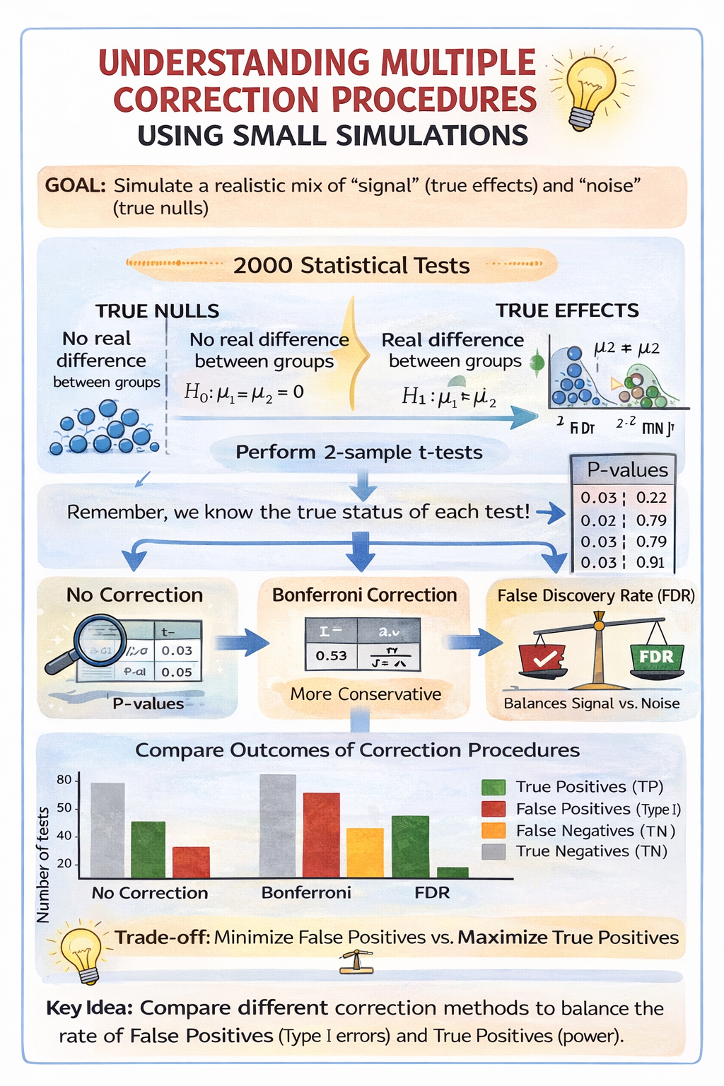
Understanding multiple correction procedures using small simulations
If you have time during the tutorial, we now simulate a situation closer to real data analysis, where some tests correspond to real effects and others do not. Half of the tests are generated with no true difference between groups (true null hypotheses), while the other half are generated with a real difference in means (true effects). Because we control how the data are generated, we know which tests should be significant and which should not. We then compare what happens when we apply no correction, the Bonferroni correction, and the False Discovery Rate (FDR) procedure.
The code below simulates a situation where you run many statistical tests, but only some of them reflect real statistical differences and the rest are true nulls. The goal is to create a dataset of P-values that contains a realistic mix of “signal” and “noise,” and then show how multiple-testing corrections (Bonferroni and FDR/BH) change the conclusions.
First, you choose the size of the simulation: n.tests is how many separate tests you will run (here 2000), n.per.group is the sample size per group for each test (here 10 observations in each of two groups), and alpha is the significance threshold (0.05). These values are not special—they are just reasonable numbers that make the simulation stable and quick.
Next, the code creates a vector called truth that encodes which tests truly have an effect and which do not. In this example, half the tests are assigned 0 (meaning “no real difference between the two groups”) and half are assigned 1 (meaning “there is a real difference”). This is the key advantage of simulation: unlike real studies, we know which hypotheses are actually true or false.
Then the code generates the P-values. For each entry of truth, it creates two groups of random data (x1 and x2). Group 1 is always generated with mean 0. Group 2 is generated with mean equal to eff, where eff is taken from truth. So, when eff = 0, both groups have the same mean and the null hypothesis is true; any “significant” result is a false positive due to sampling variation. When eff = 1, group 2 has a higher mean than group 1, so there is a true effect; if the test is not significant, that is a false negative. A two-sample t-test is then applied to each pair of groups, and the P-value is extracted and stored. The sapply function simply repeats this process efficiently across all 2000 tests and returns the full vector of P-values.
Finally, the code applies different multiple-testing strategies to those P-values. p.none keeps the original P-values (no correction). p.bonf applies the Bonferroni correction, which is very conservative and strongly reduces false positives but can miss real effects. p.fdr applies the Benjamini–Hochberg procedure (coded as “BH”), which controls the False Discovery Rate and typically keeps more power while still limiting the proportion of false discoveries among the results declared significant. These three vectors—uncorrected, Bonferroni-corrected, and FDR-corrected—can then be compared to see how many discoveries each method makes and, because we know truth, how many are true positives versus false positives.
n.tests <- 2000
n.per.group <- 10
alpha <- 0.05

# Truth: 0 = no effect, 1 = true effect
truth <- c(rep(0, n.tests/2), rep(1, n.tests/2))

# Generate p-values
p.values <- sapply(truth, function(eff) {
  x1 <- rnorm(n.per.group, mean = 0, sd = 1)
  x2 <- rnorm(n.per.group, mean = eff, sd = 1)
  t.test(x1, x2, var.equal = TRUE)$p.value
})

# Adjustments
p.none <- p.values
p.bonf <- p.adjust(p.values, method = "bonferroni")
p.fdr  <- p.adjust(p.values, method = "BH")
The next code below takes the P-values generated above and classifies the outcome of each statistical test based on two pieces of information:
whether the test was declared significant, and
whether a real effect was present in the data-generating process. The goal is to explicitly count true positives, false positives, false negatives, and true negatives for each multiple-testing procedure.
The function classify_results() does this classification. It first applies the usual decision rule of hypothesis testing: a test is considered significant if its P-value is less than or equal to the chosen significance level alpha (here 0.05). This produces a logical vector called decision that records, for each test, whether the null hypothesis was rejected or not.
The function then compares this decision to the known “truth” from the simulation. When a test is significant and a real effect exists (truth == 1), it is counted as a true positive (TP). When a test is significant but no real effect exists (truth == 0), it is a false positive (FP). When a test is not significant even though a real effect exists, it is a false negative (FN). Finally, when a test is not significant and no real effect exists, it is a true negative (TN). The function returns these four counts in a single named vector.
The function is then applied three times: once to the unadjusted P-values (p.none), once to the Bonferroni-adjusted P-values (p.bonf), and once to the FDR-adjusted P-values (p.fdr). Each call returns the number of TP, FP, FN, and TN for that specific correction method.
# decision <- p <= alpha compares each P-value in the vector p to alpha and returns a logical vector (TRUE / FALSE) of the same length. Each element indicates whether that test is declared significant.

classify_results <- function(p, truth, alpha = 0.05) {
  decision <- p <= alpha
  c(
    TP = sum(decision & truth == 1),
    FP = sum(decision & truth == 0),
    FN = sum(!decision & truth == 1),
    TN = sum(!decision & truth == 0)
  )
}

res.none <- classify_results(p.none, truth)
res.bonf <- classify_results(p.bonf, truth)
res.fdr  <- classify_results(p.fdr, truth)

results <- rbind(
  None = res.none,
  Bonferroni = res.bonf,
  FDR = res.fdr
)
results
Let’s represent the results graphically. The code below takes the summary table of results from the simulation (counts of true positives, false positives, false negatives, and true negatives) and turns it into a clear grouped barplot using ggplot2.
First, the results table is reorganized into a format suitable for plotting. A data frame is created where each row corresponds to a multiple-testing method (None, Bonferroni, FDR), and the four outcome types (TP, FP, FN, TN) are stored as separate columns. The Method variable is explicitly defined as a factor with a chosen order so that the methods appear from left to right in a logical sequence.
Next, the data are reshaped from a “wide” format (one column per outcome) into a “long” format, where each row represents a single outcome count for a given method. This long format is what ggplot expects when different categories (here TP, FP, FN, TN) are mapped to colours within the same plot.
The plotting section then builds a grouped barplot. The x-axis shows the multiple-testing method, the y-axis shows the number of tests, and the fill colour distinguishes among the four outcome types. Bars are placed side by side for easy comparison across methods. Colours are manually chosen so that correct decisions and errors are visually distinct, and the legend labels are written out explicitly to avoid ambiguity.
Finally, labels and a clean visual theme are applied. The legend is placed outside the plotting area, the axis text is emphasized for readability, and unnecessary visual clutter is removed. The resulting figure clearly shows how each multiple-testing procedure differs in terms of true positives, false positives, false negatives, and true negatives.
library(ggplot2)

# Prepare data
outcomes_df <- data.frame(
  Method = factor(rownames(results),
                  levels = c("None", "Bonferroni", "FDR")),
  TP = results[, "TP"],
  FP = results[, "FP"],
  FN = results[, "FN"],
  TN = results[, "TN"]
)

outcomes_long <- reshape(
  outcomes_df,
  varying = c("TP", "FP", "FN", "TN"),
  v.names = "Count",
  timevar = "Outcome",
  times = c("TP", "FP", "FN", "TN"),
  direction = "long"
)

# Plot
ggplot(outcomes_long,
       aes(x = Method, y = Count, fill = Outcome)) +
  geom_col(position = position_dodge(width = 0.8), width = 0.7) +
  scale_fill_manual(
    values = c(
      TP = "darkgreen",
      FP = "firebrick",
      FN = "orange",
      TN = "gray70"
    ),
    labels = c(
      TP = "True positives (TP)",
      FP = "False positives (Type I)",
      FN = "False negatives (Type II)",
      TN = "True negatives (TN)"
    )
  ) +
  labs(
    x = "",
    y = "Number of tests",
    title = "Outcomes of multiple-testing procedures"
  ) +
  theme_classic(base_size = 14) +
  theme(
    legend.position = "right",
    legend.title = element_blank(),
    axis.text.x = element_text(face = "bold")
  )
Without correction, many true effects are detected, but this comes with several false positives. The Bonferroni correction almost eliminates false positives, but at the cost of missing nearly all true effects (many false negatives). The FDR procedure lies between these two extremes: it detects more true effects than Bonferroni while keeping false positives relatively low. This illustrates the trade-off between avoiding false positives and retaining power to detect real effects.
A somewhat challenging exercise if you’re interested
In this exercise, you will explore how the results change when true effects are weaker or stronger, while keeping the number of tests and the significance threshold (alpha = 0.05) the same. Your goal is to observe how Bonferroni and FDR (BH) differ in terms of:
• False positives (FP)
• False negatives (FN)
• True positives (TP)
• True negatives (TN)
Step 1 — Make the simulation a function; this is where R is great - we can create functions that optimize the change of parameters.
Copy and paste the code below. This function runs the full simulation and returns the outcome table (results) for a chosen effect size.
run_simulation <- function(effect = 1, n.tests = 2000, n.per.group = 10, alpha = 0.05) {

  # Truth: 0 = no effect, 1 = true effect
  truth <- c(rep(0, n.tests/2), rep(1, n.tests/2))

  # Generate p-values
  p.values <- sapply(truth, function(eff) {
    x1 <- rnorm(n.per.group, mean = 0, sd = 1)
    x2 <- rnorm(n.per.group, mean = eff * effect, sd = 1)
    t.test(x1, x2, var.equal = TRUE)$p.value
  })

  # Adjustments
  p.none <- p.values
  p.bonf <- p.adjust(p.values, method = "bonferroni")
  p.fdr  <- p.adjust(p.values, method = "BH")

  classify_results <- function(p, truth, alpha = 0.05) {
    decision <- p <= alpha
    c(
      TP = sum(decision & truth == 1),
      FP = sum(decision & truth == 0),
      FN = sum(!decision & truth == 1),
      TN = sum(!decision & truth == 0)
    )
  }

  res.none <- classify_results(p.none, truth, alpha)
  res.bonf <- classify_results(p.bonf, truth, alpha)
  res.fdr  <- classify_results(p.fdr, truth, alpha)

  results <- rbind(
    None = res.none,
    Bonferroni = res.bonf,
    FDR = res.fdr
  )

  return(results)
}
Step 2 — Run the simulation for three effect sizes
Run the function for three scenarios:
• Weak effect: effect = 0.2
• Moderate effect: effect = 0.5
• Strong effect: effect = 1.0
results_weak  <- run_simulation(effect = 0.2)
results_mod   <- run_simulation(effect = 0.5)
results_strong <- run_simulation(effect = 1.0)

results_weak
results_mod
results_strong
Step 3 — Plot the outcomes (TP, FP, FN, TN)
Use the ggplot code below to visualize the results for one of your simulations (start with the moderate effect).
library(ggplot2)

plot_outcomes <- function(results_table, title_text = "Outcomes of multiple-testing procedures") {

  outcomes_df <- data.frame(
    Method = factor(rownames(results_table), levels = c("None", "Bonferroni", "FDR")),
    TP = results_table[, "TP"],
    FP = results_table[, "FP"],
    FN = results_table[, "FN"],
    TN = results_table[, "TN"]
  )

  outcomes_long <- reshape(
    outcomes_df,
    varying = c("TP", "FP", "FN", "TN"),
    v.names = "Count",
    timevar = "Outcome",
    times = c("TP", "FP", "FN", "TN"),
    direction = "long"
  )

  ggplot(outcomes_long, aes(x = Method, y = Count, fill = Outcome)) +
    geom_col(position = position_dodge(width = 0.8), width = 0.7) +
    scale_fill_manual(
      values = c(TP = "darkgreen", FP = "firebrick", FN = "orange", TN = "gray70"),
      labels = c(
        TP = "True positives (TP)",
        FP = "False positives (Type I)",
        FN = "False negatives (Type II)",
        TN = "True negatives (TN)"
      )
    ) +
    labs(x = "", y = "Number of tests", title = title_text) +
    theme_classic(base_size = 14) +
    theme(
      legend.position = "right",
      legend.title = element_blank(),
      axis.text.x = element_text(face = "bold")
    )
}

plot_outcomes(results_mod, title_text = "Moderate effect (effect = 0.5)")
Now repeat the plot for results_weak and results_strong. Note that the effect size (strength of true positives) is set when the simulation is run (via the effect argument in run_simulation()), not in the plotting function. The plotting function simply visualizes the results for a given simulation. So, you need to first run the simulation with a chosen effect size (e.g., weak, moderate, or strong) to generate the results table, and only then pass that table to the plotting function to visualize the outcomes.
Questions:
Answer in 3–6 sentences (no calculations required beyond reading your results table / plot):
- When the effect is weak (0.2), which correction method shows the largest number of false negatives?
- When the effect is strong (1.0), which method produces the most true positives (TP)?
- Based on your results, explain the main trade-off between Bonferroni and FDR (BH).
Self-check - You have done the exercise correctly if:
• Bonferroni generally shows fewer FP, but often more FN (especially when effects are weak).
• FDR (BH) generally shows more TP than Bonferroni, while keeping FP lower than the “None” method.