Tutorial 5: Rank-transformation and Heteroscedasticity

February 10, 2026
Dealing with non-normal and heteroscedastic data in ANOVA designs

CRITICAL: Regular practice with R and RStudio, the statistical software used in BIOL 322 and introduced during tutorial sessions, and consistent engagement with tutorial exercises are essential for developing strong skills in Biostatistics.

EXERCISES: Tutorial reports are independent exercises and are not submitted for grading; however, students are strongly encouraged to complete them. Some tutorials include solutions at the end to support self-assessment and review. Other tutorials do not require model answers because they are procedural and can be easily self-assessed by verifying that the code runs correctly and produces the expected type of output.

General setup for the tutorial
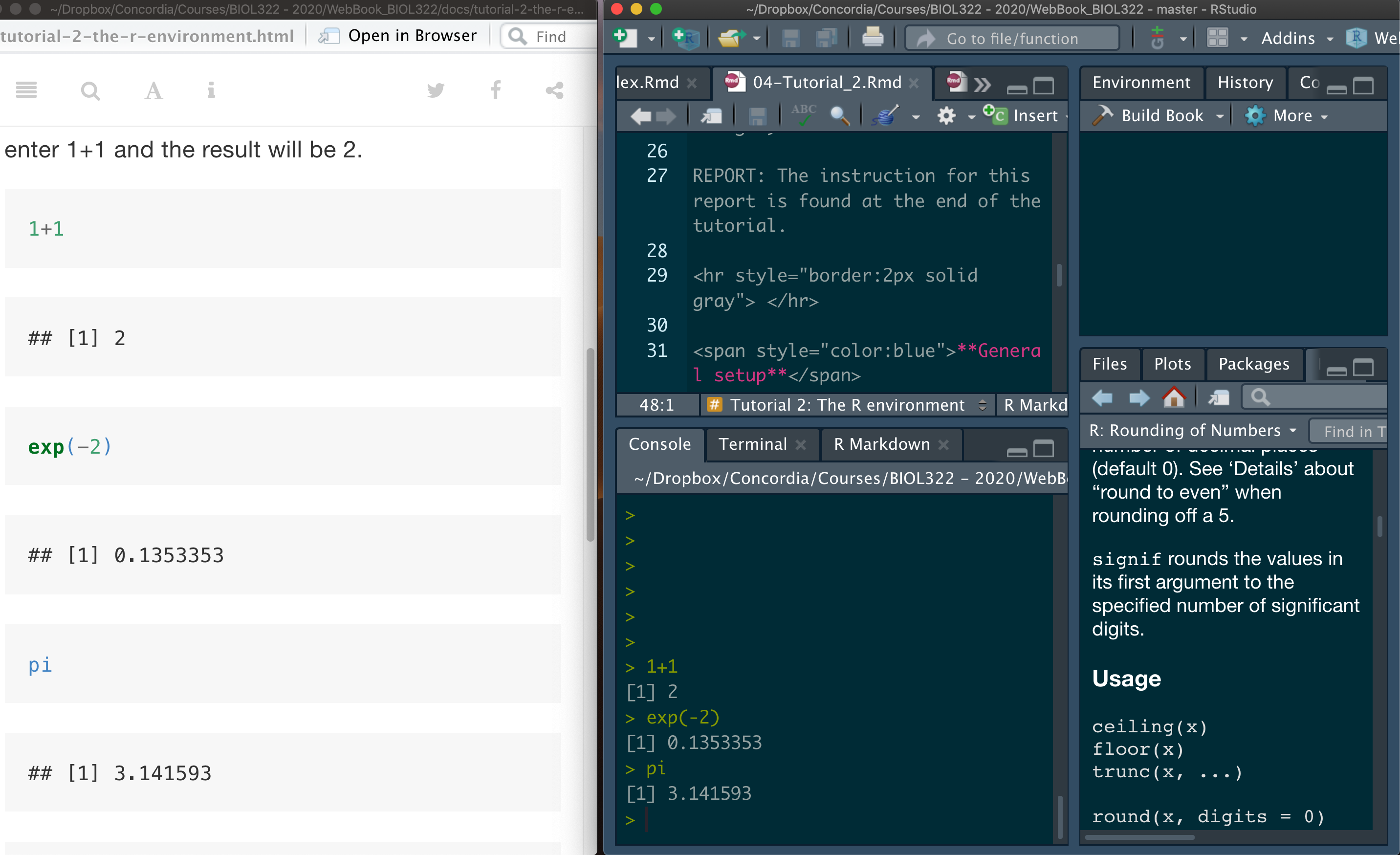
A good way to work through is to have the tutorial opened in our WebBook and RStudio opened beside each other.

*NOTE: Tutorials are produced in such a way that you should be able to easily adapt the commands to your own data! And that’s the way that a lot of practitioners of statistics use R!

Ranked transformation to tackle data that cannot be assumed to be normally distributed

As we discussed in our lectures, even though parametric tests (e.g., t-test, ANOVAs, etc) assume normality, they are quite robust when the assumption of normality is not met. That said, depending on the field of research, there is a tradition in terms of requiring that non-parametric options should be used even in cases where data are not too different from being normally distributed. One of the most widely used alternatives approaches for when data cannot be assumed to be normal are based on rank transformed data (as seen in our lectures).

Here we will use the F_st data from McDonald et al. (1996) seen in class.

Description: F_st is a measure of the amount of geographic variation in genetic polymorphism. McDonald et al. (1996) compared two populations of the American oyster using F_st estimated on six anonymous DNA polymorphisms (variation in random bits of DNA of no known function) and 13 proteins.

Question: Do protein differ in their F_st values in contrast to anonymous DNA polymorphisms?

Download the F_st data
Load the data:

Fst <- read.csv("McDonald_etal_1996.csv")
View(Fst)

Although the F_st data only have two groups (i.e., DNA and protein), this is a good place to remember that ANOVA (usually applied to data with more than two groups) and two-sample t-tests (applied to data with 2 groups) are the same. Let’s first run the ANOVA; we start by running the linear model (using function lm) where F_st values are the response (dependent) variable and factor origin (DNA or protein) is the predictor variable treated as a factor. The function as.factor transforms the code for origin in a way that the function lm runs an ANOVA instead of a standard regression. Although we can use the function aov to run the ANOVA (as seen in previous R tutorials), the function lm is more useful when running more complex analyses as we will see later in our R tutorials.

lm.Fst <- lm(Fst~as.factor(origin),data=Fst)
anova(lm.Fst)

The F-value = 0.1045 and the and P-value = 0.7502.

Note that the numerator degrees of freedom (df) is 1 because we only have two groups and the denominator df is 18 because we have 20 observations (i.e., number of F_st values) and we loose 2 degrees of freedom because the mean of each group (DNA and protein) were used to calculate their variances, which in turn are used to estimate the residuals (i.e., within group sum-of-squares as seen in our ANOVA lecture).

Now let’s calculate the two-sample (two-groups) t-test to demonstrate the relationship between the t- and the F-distributions:

t.test(Fst~as.factor(origin),data=Fst,var.equal=TRUE)

Look over the results and you will note first that the P-value is exactly the same as for the ANOVA, i.e., P-value = 0.7502, which is exactly the same as the one based on the F-distribution (i.e., ANOVA). The t-value is 0.3233. Let’s square the t-value:

0.3233^2

The squared t-value is exactly the F-value for the ANOVA calculated earlier (i.e., 0.1045). This shows that a two-sample t-test and a one-way ANOVA with two groups are mathematically equivalent tests. In fact, squaring a t statistic yields an F statistic with 1 degree of freedom in the numerator (corresponding to two groups) and n - 2 degrees of freedom in the denominator.

You might then ask why we bother learning t-tests for comparing two means if ANOVA can do the same job. The answer is largely historical and practical. The t-test was developed first as a simple, direct tool for comparing two groups, with an interpretation that is often more intuitive in that context (e.g., a signed statistic indicating the direction of the difference). ANOVA, by contrast, was developed as a general framework for comparing more than two groups, and the two-group case is simply a special (degenerate) instance of it.

In practice, both tests rely on the same assumptions and test the same null hypothesis when there are only two groups. Learning the t-test helps build intuition about mean comparisons, variability, and sampling distributions, while ANOVA provides a unifying framework that scales naturally to more complex designs. Conceptually, it is best to think of the t-test not as a different test, but as ANOVA in its simplest possible form.

A t-test asks how far apart two means are, whereas ANOVA asks whether the variability between group means is large relative to variability within groups. With just two groups, these are the same question, which is why the tests give the same result.

Now, let’s get back to our F_st example. The first step is to determine whether a parametric ANOVA is appropriate for these data. This is done by assessing whether the model residuals are approximately normally distributed, which we evaluate using a Q–Q normal residual plot.

plot(lm.Fst,which=2,col="firebrick",las = 1,cex.axis=1,pch=16)

The residuals deviate markedly from the pattern expected if the within-group errors were normally distributed. As a result, a parametric ANOVA is not appropriate, and we instead use the Kruskal–Wallis test.

kruskal.test(Fst~origin,data=Fst)

Now let’s compare the p-value from the Kruskal–Wallis test with the one obtained from an ANOVA applied to ranked (transformed) data. As we saw in class, these p-values are typically very similar because both approaches are based on the same underlying idea: replacing the raw data with their ranks.

A key practical difference, however, is that the Kruskal–Wallis test is limited to one-factor designs. In contrast, ANOVA on ranked data naturally extends to more complex designs, making it the general framework for rank-based analyses when dealing with multifactorial experiments (e.g., two-way or higher-order ANOVAs).

More broadly, rank transformation provides a general and robust strategy for handling non-normal data when the focus is on differences among groups, while still allowing the use of familiar ANOVA machinery.

In R, the function rank transforms data on ranks:

Fst.ranked<-rank(Fst$Fst)
Fst.ranked

Let’s combine the original data with the transformed data:

ranked.data <- data.frame(Fst=Fst$Fst,Fst.ranked=Fst.ranked,origin=Fst$origin)
View(ranked.data)

Now let’s conduct the ANOVA on the ranked transformed data:

lm.Fst.ranked <- lm(Fst.ranked~as.factor(origin),data=ranked.data)
anova(lm.Fst.ranked)

The Kruskal–Wallis test yields a p-value of 0.8365, very close to the p-value from the ANOVA performed on ranked data (0.8429), illustrating the close correspondence between the two approaches.

Issues caused by heteroscedasticity: the case of inflated type I errors

One important issue with ANOVA when data are heteroscedastic is that false positives occur more often than intended. When the null hypothesis is actually true, the test rejects it more frequently than the risk level you specified (i.e., \(\alpha\)). In other words, the actual Type I error rate can be higher than the nominal \(\alpha\) you chose (e.g., 0.05). This phenomenon is known as inflated Type I error.

We will begin by estimating Type I error rates under homoscedasticity and then under heteroscedasticity, so you can see how and why problems arise. We did this explicitly in Lectures 7 and 8.

Let’s assume that we sample observations from three normally distributed populations that all have the same mean (10) and the same standard deviation (30). By setting the means equal, we ensure that the null hypothesis is true.

Of course, this is a simulation designed to illustrate the issues involved. In real data analyses, we never know the true underlying conditions—specifically, whether the null hypothesis is actually true or false. However, simulations are powerful precisely because they allow us to explore how statistical tests behave when assumptions are met or violated, and to see what can go wrong if those assumptions are ignored.

Recall that the variance is the square of the standard deviation. We then test, using a one-way ANOVA, whether the group means differ. This procedure is repeated 10 000 times, and the p-value from each ANOVA is recorded.

We then count how often the ANOVA null hypothesis is rejected—that is, how often we incorrectly conclude that at least two group means differ. The sample size in each group is fixed at 20 observations, although in practice group sizes may differ. Finally, we set the significance level to \(\alpha\) = 0.05.

Groups <- c(rep(1,each=20),rep(2,each=20),rep(3,each=20))
Groups
alpha <- 0.05
n.tests <- 10000
data.simul <- data.frame(replicate(n.tests,c(rnorm(n=20,mean=10,sd=30),rnorm(n=20,mean=10,sd=30),rnorm(n=20,mean=10,sd=30))))
dim(data.simul)

Note that the simulated data consist of 60 rows (i.e., 60 values coming from three groups of 20 observations each, 20 \(\times\) 3 = 60) and 10 000 columns, with each column representing one simulated dataset. Each of these 10 000 datasets is then analyzed using a one-way ANOVA as described below. This step may take a little while to run (about 2–3 minutes).

This will take less than a minute depending on your computer:

lm.results <- lapply(data.simul, function(x) {
  lm(x~Groups, data = data.simul)
})
ANOVA.results <- lapply(lm.results, anova)

We now extract the p-value from each ANOVA. Because this is a one-factor (one-way) ANOVA, each model returns a single p-value testing for differences among group means. The code below collects those p-values across all simulations and then estimates the Type I error rate by calculating the proportion of tests (over 10 000) that are significant at \(\alpha\) = 0.05.

P.values <- sapply(ANOVA.results, function(x) {x$"Pr(>F)"[1]})
TypeIerror.rate <- length(which(P.values<=0.05))/n.tests # 10000
TypeIerror.rate

What did you notice? The estimated Type I error rate is close to the nominal \(\alpha\) = 0.05, as expected when model assumptions are satisfied. If we could perform an infinite number of tests, then the estimated Type I error rate would converge exactly to the nominal significance level, \(\alpha\), that was used to assess each p-value (i.e., \(\alpha\)=0.05).

Let’s plot the frequency distribution of p-values:

hist(P.values,col="firebrick")

Notice that the histogram of p-values is approximately uniform. This is the expected pattern when the null hypothesis (H₀) is true and model assumptions are satisfied, as we saw in the FDR module in Lecture 6.

The case of heteroscedasticity when the null hypothesis is true. Now let’s assume we sample observations from three normally distributed populations that all share the same mean (set to 10, so H₀ is true) like we did above, but have different standard deviations: 3, 30, and 300, respectively. We will keep the sample size the same in each group. So, unlike the case above, this data are heteroscedastic.

Groups <- c(rep(1,each=20),rep(2,each=20),rep(3,each=20))
Groups
n.tests <- 10000
data.simul <- data.frame(replicate(n.tests,c(rnorm(n=20,mean=10,sd=3),rnorm(n=20,mean=10,sd=30),rnorm(n=20,mean=10,sd=300))))
dim(data.simul)
lm.results <- lapply(data.simul, function(x) {
  lm(x~Groups, data = data.simul)
})
ANOVA.results <- lapply(lm.results, anova)
P.values <- sapply(ANOVA.results, function(x) {x$"Pr(>F)"[1]})
alpha <- 0.05
TypeIerror.rate <- length(which(P.values <= alpha))/n.tests
TypeIerror.rate

The estimated Type I error rate is much higher than the nominal significance level, at around 0.11. In other words, because the variances of the populations from which the samples were drawn differ (i.e., the populations are heteroscedastic), the nominal \(\alpha\) = 0.05 no longer reflects the true Type I error rate of the test.

As a consequence, if we were to analyze data from these populations using a standard ANOVA, we would incorrectly reject a true null hypothesis in about 11% of cases—more than twice the false-positive rate we were willing to accept when setting \(\alpha\) = 0.05.

As a result, the risk of false positives (i.e., Type I error) is much higher than the level we initially allowed (= 0.05, or 5%). It is important to note, however, that the magnitude and even the direction of this bias depend on how population variances differ: the Type I error rate can be either inflated or deflated. The key takeaway is that when data come from heteroscedastic populations, we can no longer trust that the nominal \(\alpha\) reflects the true Type I error rate of an ANOVA.

The demonstrations in this section of the tutorial is a way to help you understand critical points we covered in lectures 7 and 8 about statistical inference:

1. Statistics is conditional, not absolute: Statistical inference does not reveal biological truth; it quantifies evidence under explicit assumptions about models and sampling. Because this reasoning is conditional and probabilistic, it often clashes with our more intuitive, mechanism-focused way of thinking.

2.Non-intuitive concepts of statistical error in statistical inference: Type I and Type II errors describe how a statistical decision rule behaves across many hypothetical repetitions under uncertainty, relative to an unseen truth. Statistics therefore does not tell us whether a particular result is right or wrong; it tells us how risky our decisions would be if we repeatedly analyzed new samples drawn from the same underlying population using the same model, assumptions, and decision threshold.

Conclusion: Statistical conclusions are statements about statistical evidence given ASSUMPTIONS, not absolute claims about biological truth.

Even though all samples were drawn from populations with the same mean (so H₀ is true), the distribution of p-values is no longer uniform. Instead, it is right-skewed, with more small p-values than expected, revealing how heteroscedasticity biases ANOVA toward false positives.

hist(P.values)

As you can see, heteroscedasticity breaks the reference distribution of the test statistic, so p-values are no longer uniformly distributed under the null hypothesis; in the case here, there is an excess of smaller p-values. However, depending on the level of heteroscedasticity, we can also get an excess of large p-values (> 0.8).

Issues caused by heteroscedasticity: the case of reduced statistical power

As we discussed in lecture, when the ANOVA null hypothesis is false (i.e., at least two group means truly differ), heteroscedasticity can reduce statistical power—meaning false negatives become more common.

We will not demonstrate this computationally here. Instead, you will explore it in Report 2 by setting up a simulation in which (1) group means differ (so H₀is false) and (2) group variances are unequal (heteroscedasticity). The code used above can be modified straightforwardly to create this scenario.

Some solutions for heteroscedasticity

1) Welch’s ANOVA on ranks: As discussed in class, there are several ways to handle heteroscedasticity in ANOVA-type designs. Here we will focus on two approaches that are commonly used in biology.

The first is Welch’s one-way ANOVA, which is designed for unequal variances. In R, this is implemented with oneway.test(), using var.equal = FALSE, which applies Welch’s correction to the test’s degrees of freedom to account for heteroscedasticity.

Here, we will apply Welch’s ANOVA to the FST data.

oneway.test(Fst.ranked~origin, var.equal = FALSE,data=ranked.data)

Notice that the p-value from Welch’s ANOVA (0.8732) is slightly larger than those obtained from the Kruskal–Wallis test (0.8365) and the rank-based ANOVA (0.8429). This difference arises because Welch’s test is more conservative: it adjusts the degrees of freedom to account for unequal variances, which generally makes rejecting H₀ more difficult and therefore yields larger p-values.

Because heteroscedasticity tends to inflate Type I error rates (i.e., increase the risk of false positives), Welch’s ANOVA counteracts this problem by being deliberately cautious, reducing the likelihood of incorrectly rejecting a true null hypothesis.

For example, suppose you choose = 0.05 (5%) as the threshold for deciding whether to reject H₀. This represents the expected Type I error rate when the model assumptions are satisfied—namely, normally distributed errors and homoscedasticity (i.e., equal variances across populations).

However, when data are heteroscedastic, more than 5% of tests may be declared significant even when H₀ is true, leading to an excess of false positives, as we saw above. Welch’s ANOVA addresses this problem by being more conservative: it adjusts the test so that p-values tend to be larger, thereby reducing the probability of incorrectly rejecting a true null hypothesis (H₀).

2) Weighted least squares: Another way to address heteroscedasticity is to incorporate weights into the regression framework, an approach known as weighted least squares (WLS), as we saw in Lecture 8. The key advantage of WLS is that it naturally generalizes to multifactor ANOVAs and regression models. In contrast, Welch’s ANOVA is limited to single-factor (one-way) designs.

To understand what the WLS approach does, it helps to begin with an alternative way of assessing homoscedasticity, beyond Levene’s test. As we saw in lecture, one diagnostic approach is to examine whether the square root of the absolute values of the standardized ANOVA residuals is independent of the model’s predicted values.

This relationship can be assessed visually using the following procedure. (If you are curious about how this diagnostic plot is generated in more explicit R code, see the Miscellanea section (#1) at the end of this tutorial.)

plot(lm.Fst.ranked,which=3)

You can see that the residual variances differ markedly among the groups (here, the fitted values correspond to each group), which causes the magnitude of the residuals to depend on the predicted values. In the context of ANOVA, these predicted values represent the group-specific mean \(F_{\mathrm{ST}}\) values.

When the red smoothing line deviates systematically from a horizontal line (i.e., shows a clear trend rather than remaining flat), this indicates heteroscedasticity—because the spread of residuals changes as a function of the fitted values.

Although many biologists might simply analyze the original data, we use the rank-transformed data here because the Q–Q plot for the \(F_{\mathrm{ST}}\) values indicated a departure from normality.

To reduce heteroscedasticity in the rank-transformed data, we fit the model using weights equal to the reciprocal of the group residual variances (i.e., \(1/\text{group residual variance}\), as discussed in Lecture 8). Under this weighting scheme, groups with larger residual variance contribute less to the estimation of model parameters, whereas groups with more precise measurements contribute more. This weighted fitting procedure is known as weighted least squares (WLS).

The easiest way to perform WLS using reciprocal group residual variances—that is, using weights equal to \(1/\text{variance}\), so that groups with larger variance receive less weight—is to rely on the nlme package. If you are curious to see how the same procedure can be implemented using more “standard” R code, see the Miscellanea section (#2) at the end of this tutorial.

Installing and loading nlme:

install.packages("nlme")
library("nlme")

Now, let’s fit the WLS model using the function gls in nlme

mod.wls = gls(Fst.ranked ~ factor(origin), data=ranked.data, weights=varIdent(form= ~ 1 | origin))
summary(mod.wls)

Notice that the p-value associated with the effect of origin on \(F_{\mathrm{ST}}\) in the WLS analysis (p = 0.8702) is very close to the value obtained from Welch’s ANOVA (p = 0.8732). This agreement is expected, as both approaches explicitly account for heteroscedasticity.

Importantly, unlike Welch’s ANOVA, which is limited to single-factor designs, WLS naturally extends to multifactor ANOVAs and regression models. For this reason, WLS provides a general and flexible framework for addressing heteroscedasticity in practice.

WLS based on estimated variances per group is often called a two-stage estimation because it fits two-models:

The regular ANOVA model to estimate group residual variances (see Miscellanea);
A WLS model using the information on residual variances per group from the first fit.

More importantly, the WLS procedure can be also used for ANOVA designs in which data are distributed normally but variances vary among groups. In this case, instead of using the ranked transformed data, simply apply the WLS on the raw data instead.

Assessing the performance of Weighted Least Square under heteroscedasticity

We will use a similar simulation set up as we did earlier in this tutorial where data are simulated under heteroscedasticity (different variances or standard deviations). We will assume here that the null hypothesis is true for means and that groups will vary in variances. We will consider 3 groups and 20 observations per group:

Groups <- c(rep(1,each=20),rep(2,each=20),rep(3,each=20))
Groups

Unfortunately, the function sapply is extremely slow when dealing with object generated by the gls function from package nlme to conduct WLS. We will use a for loop that improves on speed (sapply is a wrapper for loops anyway). for loops are at the core of any programming environment and has a multitude of applications. Results will be kept in a list that can be created as follows:

wls.results <- list()

Run the for loop; this may take a minute or so:

n.tests <- 1000
for (count.data.sets in 1:n.tests){
    data.simul <- c(rnorm(n=20,mean=10,sd=3),rnorm(n=20,mean=10,sd=30),rnorm(n=20,mean=10,sd=300))
    wls.results[[count.data.sets]] <- gls(data.simul ~     
         factor(Groups), weights=varIdent(form= ~ 1 | Groups))
}

The result for each WLS analysis based on the gls function is kept in the list wls.results. Each result and the associated ANOVA can be run calling the appropriate data set. For instance, for the third simulated data we simply:

wls.results[[3]]
anova(wls.results[[3]])

To estimate the Type I error rate, we only need the p-value from each ANOVA. The code below shows how to extract that value directly from the ANOVA table.

anova(wls.results[[3]])$"p-value"[2]

Let’s run now the ANOVA for all the gls models and estimate the type I error:

ANOVA.results <- lapply(wls.results, anova)
P.values <- sapply(ANOVA.results, function(x) {x$"p-value"[2]})
alpha <- 0.05
TypeIerror <- length(which(P.values <= alpha))/n.tests
TypeIerror

You will notice that the estimated Type I error rate is close to 0.05, although in some cases it may be slightly higher (e.g., around 0.06). This small deviation is expected because we are working with a finite number of simulated datasets (1 000, not an infinite number). We can also change the weights. Here we used weights=varIdent(form= ~ 1 | Groups). This works well if heteroscedasticity is mainly between groups, which is the case we simulated. There are many possibilities of weights depending on the situation.

There are many possible variance structures depending on the biological context. For example, when variability increases or decreases with the mean, a common pattern in ecological data, we could instead use weights = varPower(form = ~ fitted(.)). This allows the residual variance to scale with the mean. This was not appropriate for our simulated data because all group means were equal, but the following example illustrates how such a structure would be used in practice. But here is an example:

data.simul <- c(rnorm(n=20,mean=10,sd=3),rnorm(n=20,mean=10,sd=30),rnorm(n=20,mean=10,sd=300))
wls.results <- gls(data.simul ~     
         factor(Groups), weights = varPower(form = ~ fitted(.)))
anova(wls.results)

Again, there are many different ways to set these weights and they will differ depending on the way variance changes among groups. The key point is that this simulation demonstrates, in a computationally explicit way, that the inflated Type I error caused by heteroscedasticity can be effectively controlled using WLS.

Let’s plot the frequency distribution of p-values:

hist(P.values)

Note that it is much more uniform than for when we used the standard ANOVA approach on heteroscedastic data.

Observation: In the next tutorial, we will see an example of WLS for a two-factorial ANOVA and for post-hoc tests to compare means as well.

Miscellanea:

part 1

Code to reproduce plot(ranked.ols,which=3) as used above. Instead of using the standard R function, we are doing the calculations involved and then plotting. This should help understanding how the plot works.

plot(sqrt(abs(scale(lm.Fst.ranked$residuals)))~lm.Fst.ranked$fitted)
abline(lm(sqrt(abs(scale(lm.Fst.ranked$residuals)))~lm.Fst.ranked$fitted),col="red",ylim=c(0,1.2))

part 2

How to run WLS using more “standard” R code instead of the gls function. This will hopefully allow you to understand a bit better what WLS does; as we saw in our lecture.

2.1) Calculate the residual variance per group (i.e., origin)

var.per.origin<-aggregate(lm.Fst.ranked$residuals,list(as.factor(ranked.data$origin)),var)
var.per.origin

2.2) Duplicate variances respecting the order of origin in the data:

var.vector <- vector()
var.vector[which(ranked.data$origin=="DNA")] <- 66.44167
var.vector[which(ranked.data$origin=="Protein")] <- 25.40797
var.vector

Run the ANOVA using the standard lm function as used to conduct ANOVAs:

lm.Fst.WLS <- lm(Fst.ranked~as.factor(origin), weights = 1/var.vector, data=ranked.data)
summary(lm.Fst.WLS)

Now using the gls function

gls.result <- gls(Fst.ranked~as.factor(origin), weights=varIdent(form= ~ 1 | origin),data=ranked.data)
anova(gls.result)

Note that the p-values from summary(lm.Fst.WLS) and anova(gls.result) are the same!

Exercise

Controlled heteroscedasticity: In this exercise, you will use simulations to explore how increasing levels of heteroscedasticity affect statistical inference when the null hypothesis is true. Simulate data from three groups with equal means (e.g., mean = 10 for all groups) and equal sample sizes (e.g., 20 observations per group), but progressively increase the differences in variance among groups. For example, start with a homoscedastic scenario in which all groups have the same standard deviation (e.g., SD = 10), then move to moderately heteroscedastic data (e.g., SD = 10, 20, 40), and finally to strongly heteroscedastic data (e.g., SD = 10, 30, 300).

For each scenario, run a standard one-way ANOVA across a large number of simulated datasets (at least 1 000 repetitions), record the p-values, and estimate the Type I error rate using \(\alpha\) = 0.05. Plot the frequency distribution of p-values for each case and compare how the distribution changes as heteroscedasticity becomes more severe. Use these results to assess how violations of the equal-variance assumption influence both the shape of the p-value distribution and the reliability of statistical inference.

Answer: The goal is to keep the null hypothesis true (equal means across groups) while progressively increasing heteroscedasticity (unequal variances). For each scenario, we simulate many datasets, run a one-way ANOVA for each dataset, extract the p-values, estimate the Type I error rate as the proportion of p-values ≤ 0.05, and then plot the p-value histogram.

To make the workflow clean and reproducible, we first define a small function called simulate_anova_pvalues() that (a) simulates the data and (b) returns the p-values and Type I error rate estimates.

alpha <- 0.05
n.tests <- 10000   # increase to 30000 if you want smoother histograms
n.per.group <- 20

Groups <- factor(rep(1:3, each = n.per.group))

simulate_anova_pvalues <- function(sds, mean.value = 10, n.tests = 2000, n.per.group = 20, alpha = 0.05){
  
  # Create group labels (fixed design)
  Groups <- factor(rep(1:3, each = n.per.group))
  
  # Simulate n.tests datasets; each column is one dataset of length 60
  data.simul <- data.frame(replicate(n.tests, c(
    rnorm(n.per.group, mean = mean.value, sd = sds[1]),
    rnorm(n.per.group, mean = mean.value, sd = sds[2]),
    rnorm(n.per.group, mean = mean.value, sd = sds[3])
  )))
  
  # Run ANOVA for each dataset and extract the single p-value
  lm.results <- lapply(data.simul, function(x) lm(x ~ Groups))
  anova.results <- lapply(lm.results, anova)
  p.values <- sapply(anova.results, function(tab) tab$"Pr(>F)"[1])
  
  # Type I error estimate
  typeI <- mean(p.values <= alpha)
  
  return(list(p.values = p.values, typeI = typeI))
}

Now we define the three variance scenarios. The first is homoscedastic (all SDs equal). The second and third introduce moderate and strong heteroscedasticity, respectively:

scenarios <- list(
  homoscedastic = c(10, 10, 10),  
  moderate_hetero = c(10, 20, 40), # smaller heteros
  strong_hetero = c(10, 30, 300)
)

Next, we run the simulation for each scenario and store the results. This will take a little while to generate (more than a minute) given that we’re using 10 000 simulated data sets as set earlier.

results <- lapply(scenarios, function(sds){
  simulate_anova_pvalues(sds = sds, mean.value = 10, n.tests = n.tests,
                         n.per.group = n.per.group, alpha = alpha)
})

# Print Type I error estimates
sapply(results, function(x) x$typeI)

You should observe that the homoscedastic scenario produces a Type I error rate close to 0.05 (allowing small deviations due to finite simulation), while the heteroscedastic scenarios can produce Type I error rates that depart substantially from 0.05.

Finally, we plot the p-value histograms. Under the true null hypothesis and correct assumptions, p-values should be approximately uniform. Departures from uniformity indicate that the test is no longer behaving as intended.

par(mfrow = c(1, 3), las = 1)

hist(results$homoscedastic$p.values,
     main = "Homoscedastic\nSD = 10, 10, 10",
     xlab = "p-values")

hist(results$moderate_hetero$p.values,
     main = "Moderate heteroscedasticity\nSD = 10, 20, 40",
     xlab = "p-values")

hist(results$strong_hetero$p.values,
     main = "Strong heteroscedasticity\nSD = 10, 30, 300",
     xlab = "p-values")

par(mfrow = c(1, 1))

As you can see, heteroscedasticity breaks the reference distribution of the test statistic, so p-values are no longer uniformly distributed under the null hypothesis. Once that happens, you don’t just get too many small p-values; you get too much probability mass at both extremes.

You will also notice that under heteroscedasticity and when the null hypothesis is true (i.e., no mean differences among groups), the test statistic no longer follows the theoretical F distribution. That means:

Some datasets exaggerate signal → small p-values (Increase type I error rate overall).
Some datasets exaggerate noise → large p-values.
Middle p-values (around 0.5) become less common in comparison to small and large p-values.

The problem is really the small p-values that are in greater proportion than 0.05, which is the \(\alpha\) level set by us in terms of the risks of false positive that we can accept.