Lecture 17: post-hoc ANOVA
March 27, 2026post-hoc ANOVA analysis
When the null hypothesis of an ANOVA is rejected, we accept the alternative hypothesis, which states that “at least two samples come from different statistical populations with different means.” However, ANOVA does not specify which pairs of means are significantly different. Identifying these differences is a crucial step in further interpreting the outcomes of research studies.
This additional analysis is referred to as a post-hoc test, conducted after the ANOVA has been performed. Additionally, we emphasize the importance of verifying that the assumption of homoscedasticity holds before proceeding with an ANOVA, as this ensures the validity of the analysis.
Lecture
Download lecture: 3 slides per page and outline
Download lecture: 1 slide per page
Supplement to the lecture (demonstration of principles involving family-wise Type I error using code)
The computational demonstration presented here helps further illustrate the concepts discussed in this lecture.
We saw that if we set α = 0.05, meaning an acceptance region of 95% (0.95), then the probability of obtaining at least one significant result purely by chance—when no true effect exists (i.e., committing at least one Type I error or false positive)—across 24 tests is:
\[1-0.95^{24}=0.708011\]
The code below reproduces the plot showing how the probability of committing at least one Type I error increases as a function of the number of tests. It turns out that reaching a probability arbitrarily close to 100% requires at least 328 tests.
## [1] 0.9999999 0.9999999 0.9999999 1.0000000plot(n.tests,prob.atLeast1.TypeIerror,pch=16,col="firebrick",
cex=0.3, xlab="number of tests",ylab="prob. of at least one type I error")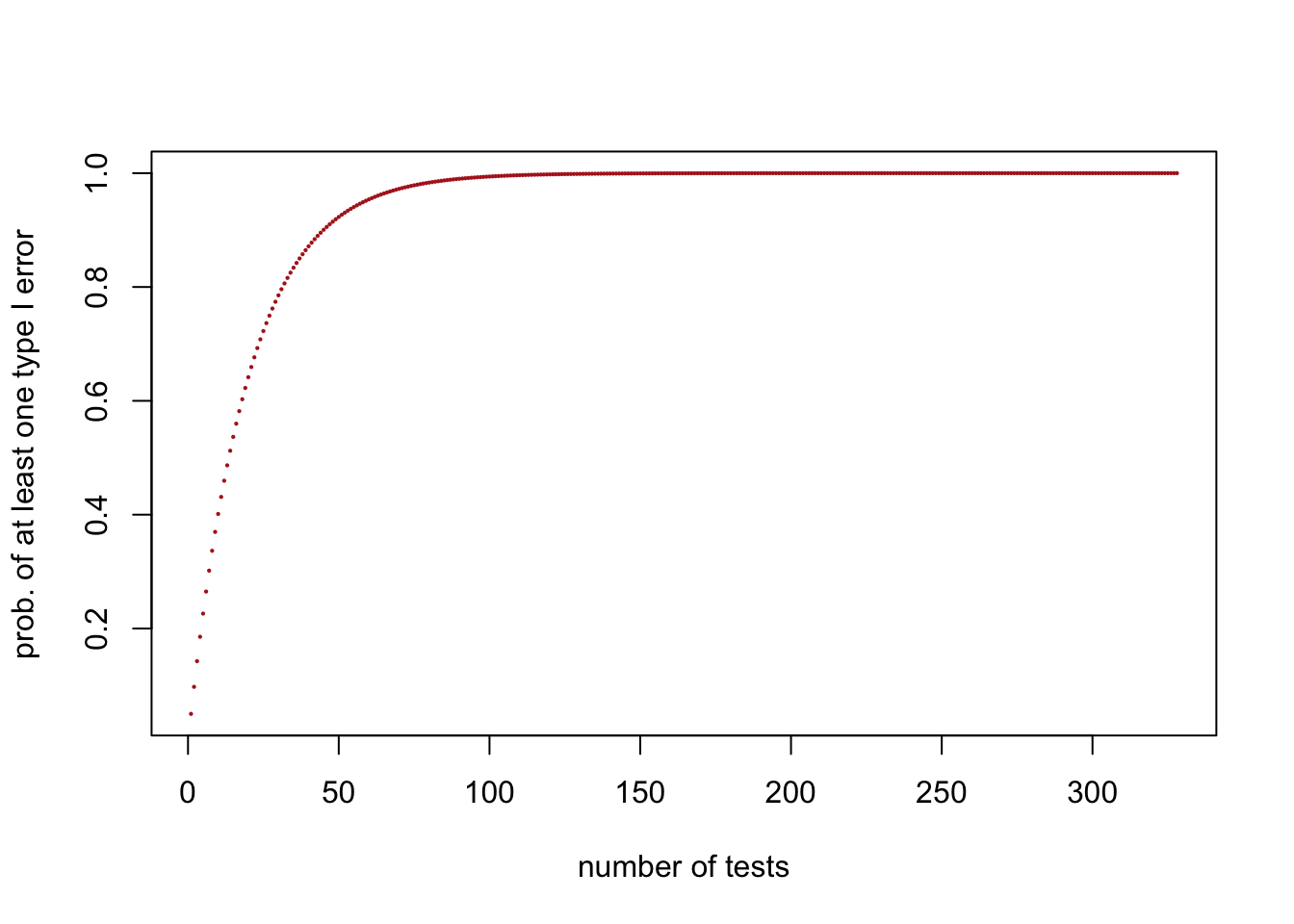
The code below generates 328 two-sample t-tests, where both samples in each test are drawn from the same population. In this case, any significant result represents a false positive (i.e., a Type I error). The set of 328 two-sample t-tests is then repeated 1000 times. For each repetition, the number of significant p-values is counted and recorded in the vector number.TypeIerrors.
This code will be relatively slow (about 5 minutes) because it performs a large number of statistical tests. Specifically, it runs 328 two-sample t-tests, repeated 1000 times, resulting in 328,000 t-tests in total. Each t-test involves computing summary statistics and p-values, which adds computational overhead. As a result, the cumulative cost of running many tests makes the simulation relatively time-consuming:
number.samples <- 328
groups <- c(rep(1,15), rep(2,15))
number.TypeIerrors <- replicate(1000, {
samples.H0.True <- replicate(number.samples, rnorm(n = 30, mean = 10, sd = 3))
p.values <- apply(
samples.H0.True,
MARGIN = 2,
FUN = function(x) t.test(x ~ groups, var.equal = TRUE)$p.value
)
sum(p.values <= 0.05)
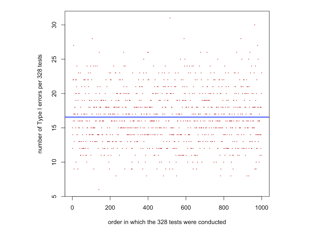
})The code below plots the number of Type I errors obtained in each set of 328 two-sample t-tests, in the order in which they were performed. The blue line shows the average number of Type I errors estimated from the simulations, given by mean(number.TypeIerrors). This value should be very close to 16.4, which is the expected number of false positives calculated as 0.05 × 328 = 16.4.
In other words, when α = 0.05, about 5% of tests are expected, on average, to be significant purely by chance, even when no true effect exists. This accumulation of false positives across multiple tests is related to what we discussed in the lecture as family-wise Type I error.
The value of mean(number.TypeIerrors) is not exactly equal to 0.05 × 328 because it is estimated from a finite number of simulations (1000 sets of 328 tests). If we repeated the simulations an infinite number of times, the estimated average would converge exactly to the theoretical expectation.
The expected number of false positives calculated as 0.05 × 328 = 16.4 is marked in the graph below as a blue horizontal line.
plot(1:1000,number.TypeIerrors,pch=16,col="firebrick",cex=0.3,xlab="order in which the 328 tests were conducted",ylab="number of Type I errors per 328 tests")
abline(h=mean(number.TypeIerrors),col="blue",lwd=2)
expected.avg.typeIerror <- 0.05*328
mean(number.TypeIerrors)