Tutorial 5: Sampling variation
Sampling variation, uncertainty, sampling properties of the mean and standard deviation, the standard error of the mean and confidence intervals
February 11 to 13, 2026
How the tutorials work
CRITICAL: Regular practice with R and RStudio, the statistical software used in BIOL 322 and introduced during tutorial sessions, and consistent engagement with tutorial exercises are essential for developing strong skills in Biostatistics. R tutorials will take place during the scheduled lab sessions.
EXERCISES: Each tutorial contains independent exercises and are not submitted for grading; however, students are strongly encouraged to complete them. Some tutorials include solutions at the end to support self-assessment and review. Other tutorials do not provide model answers because the exercises are procedural and can be easily self-assessed by checking that the code runs correctly and produces the expected type of output.
Your TAs
Section 0201: We 1:15pm-4:00pm, L-CC-213 - Sara Palestini (sarapalestini@gmail.com)
Section 0202: Th 1:15pm-4:00pm, L-CC-213 - Sara Palestini / Tristan Kolla
Section 0203: Fr 1:15pm-4:00pm, L-CC-203 - Snigdho Dutta (snigdhodeb29@gmail.com)
Section 0204: Fr 1:15pm-4:00pm, L-CC-213 - Tristan Kolla (tristan.kolla@mail.concordia.ca)
General Information
Please read the entire text carefully, without skipping any sections. The tutorials are centered on R exercises designed to help you practice understanding, performing, and interpreting statistical analyses and their results.
We have extensive experience with tutorials, and they are structured to ensure that students can complete them by the end of the session.
This particular tutorial will guide you in developing more skills in plotting with R as well.
Note: At this point we are probably noticing that R is becoming easier to use. Try to remember to:
- set the working directory
- create a RStudio file
- enter commands as you work through the tutorial
- save the file (from time to time to avoid loosing it) and
- run the commands in the file to make sure they work.
- if you want to comment the code, make sure to start text with: # e.g., # this code is to calculate…
General setup for the tutorial
An effective approach is to have the tutorial open in our WebBook alongside RStudio.
Critical notes for this tutorial
While memorizing R commands is not necessary, general concepts learned in the tutorials may be tested in exams. For example, you may be asked to explain how a computational approach can be used to build understanding about statistics, such as properties of estimators and uncertainty (see below for details).
This tutorial is designed to help you understand the nature and characteristics of sampling variation and sampling distributions. As discussed in previous Lectures (7, 8, & 9), sampling distributions are essential for understanding and making statistical inferences.
In this tutorial, we will focus on the sampling distribution of the mean and the sampling distribution of the standard deviation, as these are the most important for statistical inference. It’s important to note that although the square root of the variance \(s^2\) is the standard deviation \(s\), the characteristics of the sampling distribution of the standard deviation are slight different from the the sampling distribution of the variance. This is explained in the pedagogical guide Estimating the standard deviation.
TIP: We strongly recommend taking notes, preferably on paper, as you work through the tutorials. This practice will help you engage more deeply with the material, promoting better understanding rather than just typing commands. I assure you that taking notes will also be beneficial during exams, as you’ll need to be familiar with the properties and characteristics of estimators (such as the mean and standard deviation, which are statistics based on samples).
Computational versus analytical approaches to build sampling distributions
To understand sampling distributions and their properties, we will construct them computationally. In classical statistics, these distributions were traditionally derived analytically using calculus. The key point is that, for the concepts covered in this tutorial—and more generally—both computational and analytical approaches lead to essentially the same results. The advantage of the computational approach is that it makes these ideas more tangible: by explicitly generating samples and observing how estimates behave, it helps build intuition about sampling variation and the distributions of estimators such as the mean, standard deviation, and variance.
Over a century ago, when the foundations of statistical inference based on sampling were first developed, computers did not exist. As a result, calculus-based (analytical) methods were the only way to derive the sampling distributions that underpin statistical inference. While these analytical approaches remain central to many areas of statistics, computational methods have become increasingly common, especially as biological questions grow more complex. Simulations now provide a practical and intuitive way to explore sampling behaviour, complementing analytical results and making statistical concepts more accessible.
The main reason we use a computational approach here, rather than an analytical one, is that it provides a more intuitive way to understand the ideas underlying sampling variation and sampling distributions, and how these concepts are used in statistical inference later in the course. This is particularly important for students without formal training in mathematics and statistics, for whom calculus-based derivations can obscure the underlying logic. In my experience, however, computational approaches are also valuable for students in statistics programs, because they make abstract results concrete and reveal how theoretical properties emerge from repeated sampling. By seeing the behaviour of estimators directly, students at all levels can develop a deeper and more durable understanding of why statistical methods work, not just how to apply them.
Analytical approaches rely on a deeper background in calculus and probability, which can obscure the core intuition at this stage. By exploring these ideas through simulation, we can focus on how estimators behave under repeated sampling, while still relying on analytical results that, in many cases, have been established for over a century. Importantly, both approaches lead to the same conclusions—a point we will demonstrate explicitly in later tutorials.
Traditionally, most basic statistical inferential methods are applied using the original methods developed analytically. Analytical approaches tend to be faster because the theoretical framework is already established, and there’s no need to recreate it each time we apply a particular statistical method for inference, unlike the computational approach we are using here.
Keep in mind that the standard error represents the variability around the sample statistic of interest (e.g., mean, standard deviation, etc.). For now, we will focus on the standard error of the mean, but you can calculate the standard error for any statistic of interest, such as the standard error of the standard deviation, variance, median, and more. The standard deviation \(s\) describes the typical (average) distance of individual observations from the sample mean. When we divide s by \(\sqrt{n}\), we are no longer describing individuals, we are describing the typical distance of sample means from the true population mean.
Let’s use a fictional example to understand the difference between standard deviation and standard error.
The first thing to keep in mind is this: the standard deviation describes variation among individual observations within a sample, whereas the standard error describes variation of a statistic (e.g., the mean or standard deviation) across repeated samples. The former is a measure of variability among individual observations within a sample, whereas the latter is a measure of uncertainty in the estimate of a parameter due to sampling variation.
Imagine you are trying to guess the true average height of all students at a university.
What does the standard deviation mean? Suppose you measure the heights of 25 students. When you look at their heights, you notice that most students are about 10 cm taller or shorter than the average height of the sample. That 10 cm tells you something important: if you randomly pick one student from this group, their height will typically differ from the sample average by about 10 cm. So here, the standard deviation is about individual observations as it describes how much people vary around the average within that sample.
What happens when you take an average? Instead of guessing the true average height using just one student, you now use the average of 25 students. From experience, you know that an average based on 25 people is more reliable than relying on a single person. But how much more reliable? If the standard deviation within the sample is 10 cm, we divide it by √25 = 5. That gives 2 cm. This 2 cm is the standard error. It tells you: if you repeatedly took random samples of 25 students and calculated their average height, those averages would typically differ from the true population mean by about 2 cm.
When you use the average height of 25 students as your best guess of the true average height of all students at the university, that guess will not be exactly right. If you repeated this process a very large number times (using calculus all possible infinite sample means would be generated), each time choosing a different group of 25 students and calculating their average, some of those averages would be slightly higher and some slightly lower than the true population average. Saying that you are “typically wrong by about 2 cm” means that most of those sample averages would fall within roughly 2 cm of the true average height. In other words, 2 cm describes the usual size of the error you should expect when using a sample mean, purely because of random sampling.
Take-home message: when we use the standard error, we are no longer describing how much people differ from one another (that’s what the standard deviation does). Instead, we are describing how far our sample average is likely to be from the true population average; that is, how wrong our guess of the true mean is expected to be purely because we relied on a sample.
Sampling variation based on a normal distribution
Whether we use an analytical or computational approach, we need to assume a form for the population distribution (i.e., the marginal distribution discussed in last week’s lectures) in order to take samples from it, often referred to as ‘drawing samples from a population’.
Since the normal distribution is well-characterized (i.e., its properties are clearly defined), we can easily generate (or draw) samples from a normally distributed population using most statistical software, including R and even Excel. Analytically, this is done using calculus. Most statistical software have built-in random sampling generators for common probability distributions such as normal, uniform, and log-normal. However, the normal distribution is the most commonly assumed, as we’ve seen in our lectures. Interestingly, as we will explore here and in future lectures, assuming that the values from a statistical population are normally distributed does not mean that if the original population isn’t normal, the statistical methods we use will be totally ineffective for inference.
Let’s start by understanding how to create a vector of random values drawn from a normal distribution. All the values generated and recorded in the vector are a single sample.
In statistics, we use the term ‘to draw random values from a normal distribution’ (or any other distribution of interest). Random sampling is assumed because each value is independent of the others (recall the principles of random sampling discussed in Lecture 7). As I often say, there is only one way for samples to be independent (random sampling), but countless ways in which they can be dependent. Assuming random sampling simplifies both analytical and computational solutions. However, if the sampling is not random, the statistical methods used for inference may become biased (we will explore this further later in the course).
In the line of code below, the argument n sets the sample size, the argument mean sets the mean of the population of interest and the argument sd sets the standard deviation of the population (remember again that the standard deviation squared \(s^2\) is the variance of a distribution). A normal distribution is defined by its mean and its variance (or standard deviation). The normal distribution used here will be treated as the true population of interest! As such, the function rnorm allows us to sample from a normally distributed population with a given mean and standard deviation set by us. Let’s draw 100 values (i.e., a sample of 100 observations, i.e., n=100) from a normally distributed population with mean \(\mu\) = 20 and a standard deviation (\(\sigma\)) = 1.
Imagine the normal distribution below represents the height distribution of trees in a forest, where the true population mean height (i.e., for all trees) is 20 meters, with a standard deviation of 1 meter. In the example below, we will randomly sample 100 trees from that forest and measure their heights. Although we are sampling a finite number of trees, the normal distribution itself is assumed to have an infinite number of observational units (i.e., an infinite number of trees). Assuming statistical populations of infinite size is common and works well for finite populations. For analytical and computational purposes, statistical populations are generally considered infinite.
sample1.pop1 <- rnorm(n=100,mean=20,sd=1)
sample1.pop1
Let’s plot the frequency distribution (histogram) of our sample and calculate the sample statistics we will be working on today:
hist(sample1.pop1)
mean(sample1.pop1)
sd(sample1.pop1)
var(sample1.pop1) #i.e., sd(sample1.pop1)^2
Let’s take another sample from the same population:
sample2.pop1 <- rnorm(n=100,mean=20,sd=1)
sample2.pop1
hist(sample2.pop1)
mean(sample2.pop1)
sd(sample2.pop1)
var(sample2.pop1) # or sd(sample2.pop1)^2
Notice how the values for the summary statistics (mean, standard deviation, and variance) varied across samples? Even though they were drawn from the same population, both the data and the summary statistics differ between samples. This illustrates the principle of sampling variation, which we discussed in Lectures 7 and 8.
Let’s now generate a sample from another population with \(\mu\) = 20 and \(\sigma\) = 5 (a larger standard deviation than the value of \(\sigma\)=1 set for the previous population above):
sample1.pop2<-rnorm(n=100,mean=20,sd=5)
sample1.pop2
Let’s plot its frequency distribution (histogram) and calculate its mean and standard deviation:
hist(sample1.pop2)
mean(sample1.pop2)
sd(sample1.pop2)
var(sample1.pop2) # or sd(sample1.pop2)^2
To improve your knowledge of R and the concepts discussed below, let’s plot where the mean value falls in the distribution using a vertical line; the argument lwd controls how thick the line is plotted.
abline(v=mean(sample1.pop2),col="firebrick",lwd=3)Let’s compare the two samples by plotting their frequency distributions (histograms) of each sample on the same graph window using the function par. We will use this function to tell R that the plot will have two rows (one for each histogram) and 1 column, i.e., par(mfrow=c(2,1)). To plot 3 histograms on the same graph window we would set the function par as: par(mfrow=c(3,1)). To plot 4 histograms instead on the same graph window, two on the top row and two on the bottom row, we would set the function par as: par(mfrow=c(2,2)).
Here, we won’t make the histograms look nice as we just want to observe their differences. Note that to be able to observe the differences between the two samples, you need to make sure that the scales of axes x and y (set by the arguments xlim and ylim) are the same:
par(mfrow=c(2,1))
hist(sample1.pop1,xlim=c(0,40),ylim=c(0,50),main="Sample from Pop. 1")
abline(v=mean(sample1.pop1),col="firebrick",lwd=3)
hist(sample1.pop2,xlim=c(0,40),ylim=c(0,50),main="Sample from Pop. 2")
abline(v=mean(sample1.pop2),col="firebrick",lwd=3)
Note that both samples have an average of about 20 m, but the trees in Sample 2 vary much more among themselves. We will return to this point later in today’s tutorial.
Once finished, set the graph parameters back to their default otherwise you will have problems generated new graphs:
dev.off()From sampling variation to sampling distributions: the case of a population with a small standard deviation
Sampling variation refers to the differences in data and summary statistics that occur from sample to sample, even when drawn from the same statistical population. A sampling distribution represents the distribution of a particular statistic (e.g., mean, variance) across a large number of samples. Analytically, this can be approximated using calculus. Computationally, we can generate it as shown below. And sampling variation is the core of uncertainty in statistics.
A sampling distribution for any summary statistic can be constructed by repeatedly drawing many samples of the same size n from the same population. In this example, the population is normally distributed with a specified mean and standard deviation, but the same logic applies to any population distribution. The sample size is kept constant because the shape and spread of a sampling distribution depend directly on n. This procedure mimics the fundamental question of statistical inference: What would my estimate look like if I had drawn a different sample of the same size from the same population?
It is very easy, computationally, to draw many samples from a given population and visualize how sample means vary. However, in practice, we usually observe only one sample related to the data of interest.
Sampling variation is therefore a theoretical framework that allows us to model (analytically or computationally) the behaviour of all possible samples we could have draw. It helps us quantify the uncertainty (standard error) in our single observed estimate (say mean) by relying on the long-run properties of repeated sampling.
We can use the function replicate to do that. Below we generate 3 random samples containing 100 observations (n=100) each from a normally distributed population with a population mean \(\mu\) = 20 and population standard deviation \(\sigma\) = 1:
happy.normal.samples <- replicate(3, rnorm(n=100,mean=20,sd=1))
happy.normal.samples
Note that the name of the matrix above can take any value. So why not happy.normal.samples?!
The dimension of the matrix is 100 observations (in rows) across 3 samples (each sample is in a different column):
dim(happy.normal.samples)Let’s calculate the sample mean for each sample. For that, we will use the function apply. Each sample is in a different column; as such, we want then the MARGIN=2, i.e., calculate for each column. If we use MARGIN=1, then means are calculated per row of the matrix instead of the column. Finally, FUN here will be the mean.
apply(X=happy.normal.samples,MARGIN=2,FUN=mean)Let’s go big now. We will take 100,000 samples—one hundred thousand samples. This will not take long to compute, and it is more than sufficient to clearly reveal the patterns we are interested in. In practice, I often use one million samples or more, but for illustrating the core principles here, 100,000 samples are more than enough.
lots.normal.samples.n100 <- replicate(100000, rnorm(n=100,mean=20,sd=1))Calculate the mean for each sample:
sample.means.n100 <- apply(X=lots.normal.samples.n100,MARGIN=2,FUN=mean)
length(sample.means.n100)
There are 100,000 sample means in the vector sample means. The frequency distribution contained in this vector of sample means (sample.means.n100) is called “the sample distribution of means”. Let’s plot this distribution:
hist(sample.means.n100)
mean(sample.means.n100)
abline(v=mean(sample.means.n100),col="firebrick",lwd=3)
Note how small the variation is among sample means! Note also how the majority of them are closer to the true population mean of 20 m. This is because the distribution is symmetric. Finally, notice that the mean of these 100,000 samples means is equal (for all purposes) to the population from which their samples were taken (i.e., \(\mu\) = 20)
Now let’s return to the more realistic situation, where we usually observe only one sample. Suppose the first sample you drew is the one you actually collected. All the other samples we generated represent possible samples that could have been drawn but were not (see Lecture 7 for details).
sample.means.n100[1]The value you obtained just above is likely a sample mean very close to the true population mean. For example, suppose your sample mean was 19.84 m. The error relative to the true population value would then be 0.16 m, or 16 cm (i.e., 20.00 - 19.84). As discussed in class, we call this error sampling error. For trees that are around 20 m tall, this is a very small error, illustrating how close a single sample mean can be to the true population mean when uncertainty is low (i.e., sample size is reasonable and variability of the population is relatively low).
Can we trust this sample mean to make inferences about the population? The answer depends on the sampling distribution of sample means; that is, on all the other samples you could have drawn from the population but did not. If most of those unobserved sample means cluster close to the true population mean, then any single sample mean you happen to observe is also likely to be close. This is precisely where the concept of uncertainty enters statistical inference. When the majority of possible samples produce similar estimates, uncertainty is low and confidence in the observed sample mean is high; when they are widely spread, uncertainty is high and any single estimate becomes less reliable.
In Lectures 7, 8, and 9, we discussed how the variation within a sample, summarized by the standard deviation, provides information about how representative that sample is of the population. In this tutorial, we build on that idea by showing how within-sample variation can be used to quantify our confidence in population-level inferences.
Note that the population we considered above has a small mean relative to its standard deviation (CV = 1/20 = 0.05 = 5%), i.e., variability of the population is relatively low and remember that we used a sample size of 100 trees, which is reasonably large.
Changing sample size.
Now let’s examine what happens when the sample size changes. Suppose we had sampled 30 trees instead of 100. Should we be just as confident in an estimate based on 30 trees as we are in one based on 100 trees? To explore this question, we will estimate the sampling distribution for a sample size of 30 trees. The population remains exactly the same as before—a normal distribution with mean 20 and standard deviation 1. The only difference is the smaller sample size, which allows us to directly assess how reducing n affects uncertainty.
lots.normal.samples.n30  <- replicate(100000, rnorm(n=30,mean=20,sd=1))
sample.means.n30 <- apply(X=lots.normal.samples.n30,MARGIN=2,FUN=mean)
Now let’s plot the two sampling distributions:
par(mfrow=c(2,1))
hist(sample.means.n100,xlim=c(18.5,21.5),main="n=100")
abline(v=mean(sample.means.n100),col="firebrick",lwd=3)
hist(sample.means.n30,xlim=c(18.5,21.5),main="n=30")
abline(v=mean(sample.means.n30),col="firebrick",lwd=3)
We can also plot their probability density functions (PDF). As seen in class, they describe the relative concentration of sample mean values across the sampling distribution. In other words, the density curve shows where sample means are more likely to occur and how tightly they cluster around the true population mean.
par(mfrow=c(2,1))

hist(sample.means.n100,
     probability = TRUE,
     xlim=c(18.5,21.5),
     main="n=100")
lines(density(sample.means.n100), lwd=3)
abline(v=mean(sample.means.n100), col="firebrick", lwd=3)

hist(sample.means.n30,
     probability = TRUE,
     xlim=c(18.5,21.5),
     main="n=30")
lines(density(sample.means.n30), lwd=3)
abline(v=mean(sample.means.n30), col="firebrick", lwd=3)
Notice that the sample mean values cluster around the true population mean (20 m). Let’s verify this explicitly by calculating the mean of all sample means—that is, the average of the sampling distribution of the mean.
mean(sample.means.n100)
mean(sample.means.n30)
Notice that, for all practical purposes, the sample means are identical to the population mean, a property of sampling distributions of the mean discussed in Lecture 8.
However, more importantly, observe that the sampling distribution (i.e., the histogram of sample means) shows greater variation among the sample means when n = 30 compared to when n = 100.
To quantify this difference in spread, we calculate the standard deviation of the sample means, which is the standard error. Because the average of the sample means is essentially the same for both sample sizes, we can directly compare their standard deviations to assess how precision changes with n.
sd(sample.means.n100)
sd(sample.means.n30)
What do these values tell us? For n = 100, the standard deviation of the sample means is approximately 0.100 m (~10 cm). This indicates that, on average, a sample mean will differ from the true population mean by about 10 cm. This is not bad considering the average height of the trees is around 20 m, right? And for n = 30, the standard deviation of the sample means is approximately 0.180 m (~18 cm). This indicates that, on average, a sample mean will differ from the true population mean by about 18 cm.
Which standard deviation is smaller? Clearly, the standard deviation of the sample means based on n = 100 trees is smaller. What does this standard deviation represent? It’s the average difference between the sample mean and the population mean. On average, the sample means based on 100 trees are closer to the true population mean (20 m) than those based on 30 trees. Of course, there may be a few samples from the n = 30 group that are closer to the true population mean than some samples from the n = 100 group, but on average, this is not the case, as the smaller standard deviation of the sampling distribution demonstrates.
Under random sampling, on average, we can be more confident that samples based on n = 100 will be closer to the true population mean than those based on n = 30. In other words, by chance alone, there’s a higher probability that a single sample mean from n = 100 will be closer to the true population mean than a sample mean from n = 30 trees.
If you’re still unsure what the standard deviation above is indicating, consider this: What is the probability that a single sample based on n = 100 will be closer to the population mean than a single sample based on n = 30 trees? The standard deviation of a single sample is sensitive to sample variation among samples. To explore this, let’s first calculate the difference between the sample mean values and the true population mean:
diff.n100 <- sqrt((sample.means.n100-20.0)^2)
diff.n30 <- sqrt((sample.means.n30-20.0)^2)
dev.off()
boxplot(diff.n100,diff.n30,names=c("n=100","n=30"))
Note, again, that there is far more variation (as expected) when samples are based on n=30 than when based on n=100. How many samples are closer to the population value then?
length(which(diff.n100 <= diff.n30))/100000So, there is about a probability of 68% that a single sample based on n=100 trees will be closer to the true population value than based on a sample size of n=30.
Conclusion. In general, we have greater certainty that any given sample mean will be close to the true population value when the sample size is larger—assuming, as always, that observations (here, trees) are randomly sampled from the population.
Because we typically observe only a single sample, we can place more trust in an estimate based on 100 trees than in one based on 30 trees. Although this conclusion was illustrated using a normally distributed population, the same principle holds for other population distributions as well (e.g., uniform, lognormal), provided the samples are drawn randomly. That said, analytical solutions implemented in statistical software are often based on normal assumptions. For non-normal distributions, the exact sampling distribution of the mean is often messy or unknown in analytical form. For example, the mean of a lognormal sample does not follow a simple, named distribution, and its variance and shape depend in complicated ways on the underlying parameters. Deriving exact results requires advanced mathematics and usually leads to expressions that are impractical to use for inference.
For a lognormal (or any other) complex types of distribution, we can always use computational methods to generate the sampling distribution of the mean (and other statistics of interest). By simulating many samples from a lognormal distribution and calculating the mean for each one, we can directly observe how sample means vary, how skewed their distribution is, and how that distribution changes with sample size. No special mathematical assumptions are required. The limitation is not computational; it is analytical. Computational methods bypass this entirely by approximating the sampling distribution numerically.
This is precisely why simulations are so powerful while learning and in practice: they allow us to study sampling variation and uncertainty for any population distribution we care about, not just the normal one.
Accuracy & Precision
Let’s put what we have learned above into the perspective of accuracy and precision.
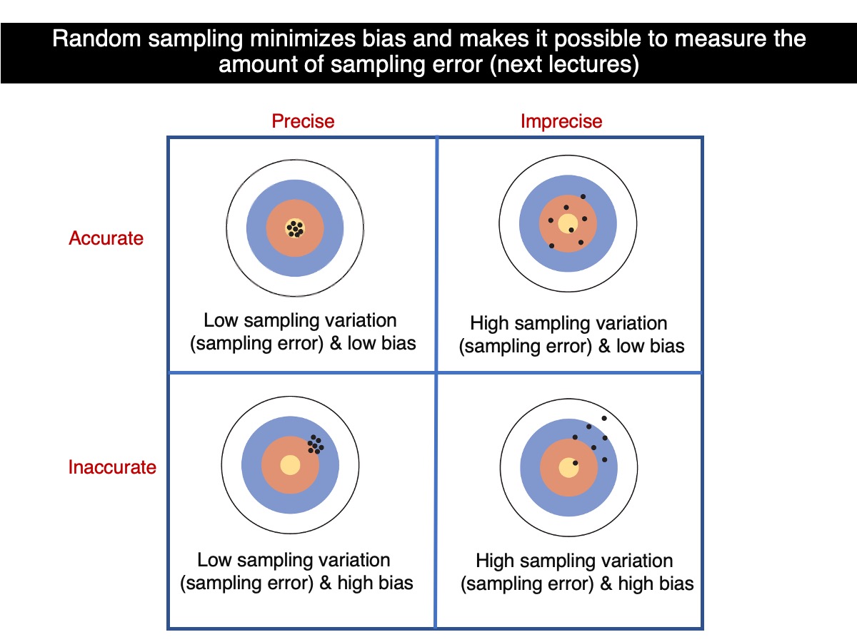
So, which sample size leads to greater precision? On average, estimates based on 100 trees are more precision than those based on 30 trees, because they tend to be closer to the true population value. Therefore, as sample size increases, bothprecision improves provided that sampling is random at all sample sizes.
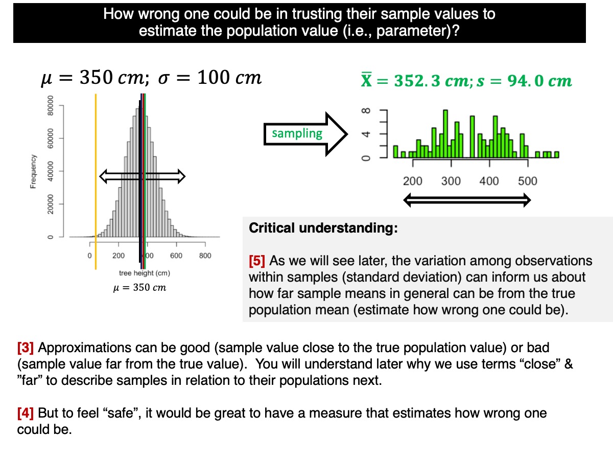
How to estimate uncertainty from one single sample?
As discussed and demonstrated in our lectures, the variation within a sample—measured by the standard deviation of the observations—provides information about how far sample means are likely to deviate from the true population mean. This expected deviation is quantified by the standard deviation of the sample means, known as the standard error.
If needed, revisit the earlier distinction between standard deviation and standard error discussed in this tutorial—the example where we estimated the average height of all students at the university.
How does that work? Let’s go back to the standard deviation of the sample distributions (i.e., among sample means):
sd(sample.means.n100)
sd(sample.means.n30)
Remember, these values are based on the variation of 100,000 sample means around the true population mean. They represent an estimate of the uncertainty (i.e., error) associated with the sample means. The standard error of the sampling distribution of means, denoted as the ‘standard error’ (\(\sigma_\bar{Y}\)), is one of the most important concepts in statistics. It quantifies how precise (a measure of uncertainty) we can estimate the true population mean. By dividing the population standard deviation by the square root of the sample size, we can calculate the standard error, which should closely match the values obtained above.
The standard error (\(\sigma_\bar{Y}\)) based on a single sample is a statistical estimate of how much sample means would vary around the true population mean if we were to repeatedly sample from the population. A lower standard error suggests that the sample mean is likely close to the population mean, indicating less uncertainty in the estimate. As the sample size increases, the standard error decreases, resulting in smaller confidence intervals and reducing uncertainty in our inference about the true population parameter. Obviously these are statistical (probabilistic expectations).
It is possible that a small sample might, by chance, produce an estimate with low uncertainty. However, this is not what we expect under random sampling. In general, however, increasing the sample size reduces sampling variation and therefore decreases uncertainty. In other words, larger samples increase the likelihood that the sample mean (or any other statistic) will be closer to the true population parameter. Again, as seen above, there is about a probability of 68% that a single sample based on n=100 trees will be closer to the true population value than based on a sample size of n=30.
cat("analytical:", 1/sqrt(100),
    "computational:", sd(sample.means.n100), "\n")
cat("analytical:", 1/sqrt(30),
    "computational:", sd(sample.means.n30), "\n")
The compuational and analytical values won’t be exactly the same; although they are very close because we used 100,000 samples. If we had used 1,000,000,000 samples, the differences would be practically imperceptible at several decimals. In the theoretical limit of an infinite number of samples, which is meaningful here because the normal distribution has infinite support via calculus, the estimated values would converge exactly to their true theoretical values for a given sample size. In other words, with infinitely many samples, there would be no error left: the sampling variability itself would remain, but our estimate of its properties would be exact.
So what does this mean in practice? We almost never know the true population standard deviation \(\sigma\). Without knowing \(\sigma\), how can we estimate how much sampling variation there is around the true population mean \(\mu\)? The answer is that we use the variability observed within the sample (i.e., the standard deviation) as a stand-in for the unknown population variability. If that variability is large, then the sample mean is expected to fluctuate more across samples, and we should be less certain about how close our estimate is to \(\mu\).
What we do instead, and remarkably, it works, is estimate that error using the standard deviation from a single sample. In other words, we use the sample standard deviation to estimate the standard deviation of the sampling variation of the mean around the true population mean \(\mu\). This is one of the most powerful ideas in statistics: from one dataset, we can quantify how uncertain our estimate is about a population value.
Let’s see how this works! Obviously there is also sampling variation around the true value of the standard deviation. So, let’s estimate standard errors from a single sample and understand how they can estimate how uncertain one can be; remember that lower uncertainty means high certainty (in average).
Let’s go back to the samples based on n=100 trees and n=30 trees. Remember that the mean of sample means equal the true population mean:
mean(sample.means.n100)
mean(sample.means.n30)
Let’s now estimate the standard deviation for each sample:
sample.sd.n100 <- apply(X=lots.normal.samples.n100,MARGIN=2,FUN=sd)
sample.sd.n30 <- apply(X=lots.normal.samples.n30,MARGIN=2,FUN=sd)
and plot their sampling distributions:
par(mfrow=c(2,1))
hist(sample.sd.n100,xlim=c(0,2),main="n=100")
abline(v=mean(sample.sd.n100),col="firebrick",lwd=3)
hist(sample.sd.n30,xlim=c(0,2),main="n=30")
abline(v=mean(sample.sd.n30),col="firebrick",lwd=3)
Boxplots could show their differences even better:
dev.off()
boxplot(sample.sd.n100,sample.sd.n30,names=c("n=100","n=30"))
Question - What did you notice?
Exercise
Write code to compare the sampling distribution of means for two normally distributed populations, both with a mean of 25 m. One population should have a standard deviation of 2 m, and the other a standard deviation of 6 m.
Next, answer the question: Which population is more likely to produce a sample mean closest to the true population mean (i.e., the parameter mean)? Use the code you developed to demonstrate your answer.
Focus solely on the sampling distributions—there’s no need to consider confidence intervals. Think (or write) a brief explanation of your answer, based on the code and the concepts covered in this tutorial.
Solution:
Both populations have the same true mean (25 m), so the center of their sampling distributions of the mean will be the same. What differs is the spread of those sampling distributions: the population with the smaller standard deviation (2 m) will produce a much tighter sampling distribution of sample means, and therefore is more likely to generate sample means close to 25 m.
## ------------------------------------------------------------
## Code solution: Sampling distributions of the mean
## Two populations with same mean but different SDs
## ------------------------------------------------------------

mu <- 25
sd_pop1 <- 2
sd_pop2 <- 6

n <- 30          # choose any fixed sample size (e.g., 30 or 100)
n_sims <- 100000 # number of repeated samples

## Draw many samples from each population
lots.samples.pop1 <- replicate(n_sims, rnorm(n=n, mean=mu, sd=sd_pop1))
lots.samples.pop2 <- replicate(n_sims, rnorm(n=n, mean=mu, sd=sd_pop2))

## Sampling distributions of the mean
sample.means.pop1 <- apply(X=lots.samples.pop1, MARGIN=2, FUN=mean)
sample.means.pop2 <- apply(X=lots.samples.pop2, MARGIN=2, FUN=mean)

## Check that both are centered ~ 25
mean(sample.means.pop1)
mean(sample.means.pop2)
Plots of both sampling distributions on the same scale:
# Common x limits to make the comparison fair
xlim.common <- range(c(sample.means.pop1, sample.means.pop2))

# Common y limits
max.freq <- max(
  hist(sample.means.pop1, plot=FALSE)$counts,
  hist(sample.means.pop2, plot=FALSE)$counts
)

par(mfrow=c(2,1))
hist(sample.means.pop1,
     xlim=xlim.common, ylim=c(0, max.freq),
     main=paste0("Sampling distribution of mean (n=", n, "), Pop. SD = ", sd_pop1),
     xlab="Sample mean", ylab="Frequency")
abline(v=mu, col="firebrick", lwd=3)

hist(sample.means.pop2,
     xlim=xlim.common, ylim=c(0, max.freq),
     main=paste0("Sampling distribution of mean (n=", n, "), Pop. SD = ", sd_pop2),
     xlab="Sample mean", ylab="Frequency")
abline(v=mu, col="firebrick", lwd=3)
Quantify which population is more likely to produce a sample mean closest to 25 m:
## ------------------------------------------------------------
## Which population is more likely to give a sample mean closest to 25?
## ------------------------------------------------------------

diff.pop1 <- abs(sample.means.pop1 - mu)
diff.pop2 <- abs(sample.means.pop2 - mu)

# Probability that Pop 1's sample mean is closer (or equally close) than Pop 2's
mean(diff.pop1 <= diff.pop2)

# Compare the spread (standard error estimated from simulations)
sd(sample.means.pop1)
sd(sample.means.pop2)
Interpretation (based on what you will see in the outputs): the population with SD = 2 m produces a much narrower sampling distribution of sample means (smaller spread), so it is more likely to yield a sample mean close to the true mean (25 m). The population with SD = 6 m produces a wider sampling distribution, so its sample means fluctuate more from sample to sample.
Extended interpretation: What happens when you take an average. Instead of guessing the true average height of all trees in the forest using one tree, you now use the average height of 25 trees. From experience, you know that an average based on 25 trees should be much more reliable than the height of a single tree, because unusually short or tall trees tend to balance out when many trees are averaged. The key question is: how much more reliable is it?
If the standard deviation of tree heights in your sample is about 1 m, that means an individual tree typically differs from the sample average by about 1 m. But when you use the average of 25 trees to estimate the true average height of the entire forest, you are no longer describing the variability of individual trees. You are describing how much the sample average would change if you had randomly selected a different set of 25 trees. Dividing 1 m by \(\sqrt{25}\) = 5 gives 0.2 m. This 0.2 m is the standard error, and it tells you:
If I use the average height of 25 trees to estimate the true average height of all trees in the forest, my estimate will typically be off by about 20 cm, purely because I relied on a sample rather than measuring every tree.