Tutorial 7: Statistical Hypothesis Testing

The principles of statistical hypothesis testing

March 11 to 13, 2026

How the tutorials work

CRITICAL: Regular practice with R and RStudio, the statistical software used in BIOL 322 and introduced during tutorial sessions, and consistent engagement with tutorial exercises are essential for developing strong skills in Biostatistics. R tutorials will take place during the scheduled lab sessions.

EXERCISES: Each tutorial contains independent exercises and are not submitted for grading; however, students are strongly encouraged to complete them. Some tutorials include solutions at the end to support self-assessment and review. Other tutorials do not provide model answers because the exercises are procedural and can be easily self-assessed by checking that the code runs correctly and produces the expected type of output.

Your TAs

Section 0201: We 1:15pm-4:00pm, L-CC-213 - Sara Palestini (sarapalestini@gmail.com)

Section 0202: Th 1:15pm-4:00pm, L-CC-213 - Sara Palestini / Tristan Kolla

Section 0203: Fr 1:15pm-4:00pm, L-CC-203 - Snigdho Dutta (snigdhodeb29@gmail.com)

Section 0204: Fr 1:15pm-4:00pm, L-CC-213 - Tristan Kolla (tristan.kolla@mail.concordia.ca)

General Information

Please read all the text; don’t skip anything. Tutorials are based on R exercises that are intended to make you practice running statistical analyses and interpret statistical analyses and results.

Note: At this point you are probably noticing that R is becoming easier to use. Try to remember to:

set the working directory
create a RStudio file
enter commands as you work through the tutorial
save the file (from time to time to avoid loosing it) and
run the commands in the file to make sure they work.
if you want to comment the code, make sure to start text with: # e.g., # this code is to calculate…

General setup for the tutorial
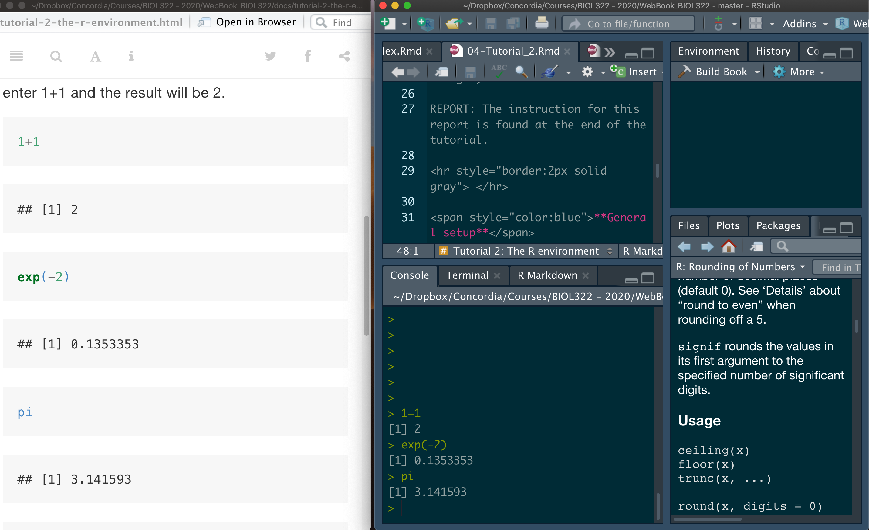
An effective way to follow along is to have the tutorial open in your WebBook alongside RStudio.

The principles of statistical hypothesis testing using a simple problem: do toads exhibit handedness?

The right hand of toads (as seen in class, but a small summary is provided here)

Statistical hypothesis testing is the most widely used framework for generating evidence in support of or against research questions or other inquiries based on data.

From Whitlock and Schluter (2014): “Humans are predominantly right handed. Do other animals exhibit handedness as well? Bisazza et al. (1996) tested this hypothesis on the common toad. They sampled (randomly) 18 toads from the wild. They wrapped a balloon around each individual’s head and recorded which forelimb each toad used to try to remove the balloon. Do other animals exhibit handedness as well?”

First step: transform the research question intoto a statistical question

From a statistical perspective, the question above can be expressed as: “Do right-handed and left-handed toads occur with equal frequency in the toad population, or is one type more frequent than the other?”

Result of the study: 14 toads were right handed and four were left handed. Are these results evidence of handedness in toads?

Do the results provide evidence that the sample value we obtained is consistent or inconsistent with samples from a theoretical population of toads, where right- and left-handed individuals occur in equal proportions? If the results are inconsistent, the data would suggest evidence that other animals exhibit handedness.

The toad component of the tutorial is in parts adapted from Whitlock and Schluter’s code on RPubs (https://rpubs.com/mdlama/153914). Since our sample consists of 18 toads, we will use this sample size to generate a sampling distribution for the theoretical population, where no limb (hand) shows dominance over the other.

We’ll begin by learning how to draw a random sample from a categorical variable with two possible outcomes, based on known probabilities (in this case, a 50/50 chance for each hand), using the desired sample size of 18 individuals.

The function below will simulate the following “manual” implementation:

The function below simulates the following ‘manual’ process:

Imagine placing millions of small pieces of paper into a bag, with half labeled ‘Left’ and the other half ‘Right.’ In practice, if we sample with replacement, only 36 pieces are needed, since any combination—such as 0 ‘Left’ and 18 ‘Right’—can occur purely by chance. (See point #2 for more explanation.)
Sample 18 pieces of paper with replacement from the bag. Sampling with replacement means that after selecting a piece, you record whether it was ‘L’ or ‘R,’ then return it to the bag before drawing the next one. This step is crucial because, without replacement, the original population’s composition would change as you sample, affecting the probabilities. For example, if your first three draws are all ‘L,’ not replacing them would increase the likelihood of drawing an ‘R’ next.

Remember, one key criterion for random sampling is independence: the selection of each individual unit (in this case, a piece of paper labeled ‘L’ or ‘R’) must not influence the selection of any other unit. This ensures that every draw is independent of the others.”

The function below is pretty self explanatory. But some details are perhaps useful. c("L", "R") sets the categories that we require; we could have written “Left” and “Right” but “L” and “R” makes the code look “simpler”. If three categories were required, we could had set them as c("A", "B","C"). size is the sample size. prob is the probability of each category. Let’s say we had 3 categories with 33.33% each as probability. Then prob = c(0.3333, 0.3333,0.333). Lastly replace = TRUE states (for the purpose of the problem here) that each observation (“toad”) has the same probability of being sample.

Sample1 <- sample(c("L", "R"), size = 18, prob = c(0.5, 0.5), replace = TRUE)
Sample1

We can then determine how many individuals in sample 1 belong to a specific category (in this case, right-handed). As you’ll see later, selecting left-handed individuals would yield the same result since the total number of individuals is fixed (i.e., 18).

sum(Sample1 == "R")

Let’s take a second sample and calculate its sum:

Sample2 <- sample(c("L", "R"), size = 18, prob = c(0.5, 0.5), replace = TRUE)
Sample2
sum(Sample2 == "R")

Most likely Sample1 and Sample2 have different numbers of right-handed individuals.

Now, let’s generate a large number of samples from the theoretical population (a computational approximation of the infinite sampling process modeled through calculus) and record the number of right-handed toads for each sample:

number.samples <- 100000
samples.n18 <- replicate(number.samples,sample(c("L", "R"), size = 18, prob = c(0.5, 0.5), replace = TRUE))
dim(samples.n18)

Let’s print the first 3 samples (remember that each sample is in a different column of the matrix samples.n18:

samples.n18[,1:3]

Let’s now calculate for each sample, the number of individuals that are right-handed:

results.n18 <- apply(samples.n18,MARGIN=2,FUN=function(x) sum(x == "R"))

The number of left-handed toads in each of the 100000 samples can be calculated simply as:

18-results.n18

Take a look into what the vector results.n18. Each value in the vector results.n18 represents the number of right-handed toads from a random sample of 18 individuals from a theoretical population in which the number of right- and left-handed toads are the same. Remember the function head lists the first 6 values in a vector or matrix:

head(results.n18)

Let’s build the frequency distribution table for the samples (i.e., sampling distribution of right-handed toads from the theoretical population):

Table.TheoreticalPop <- table(results.n18, dnn = "numberRightToads")
Table.TheoreticalPop

Note that you might not obtain any sample where all 18 individuals are right-handed or where none are right-handed (i.e., all 18 being left-handed). This is because we generated 100,000 samples, which may not be sufficient to capture every possible outcome. When I increased the sample size to 1,000,000 (one million), I observed these extreme cases.

In practice, computational methods typically involve much larger sample sizes. For analytically-based solutions (calculus-based), the distribution is modeled as though it contains an infinite number of samples. Our goal here is to provide you with the fundamental knowledge and intuition behind statistical hypothesis testing. Even with 100,000 samples, the computational approach offers a solid foundation for understanding, as it closely approximates the true distribution.

Obviously the number of samples in Table.TheoreticalPop is 100000:

sum(Table.TheoreticalPop)

We can also calculate the relative frequency of samples of different number of right-handed toads as:

Table.TheoreticalPop/100000

As expected, the most common samples are those where half of the individuals are right-handed and the other half left-handed. However, many samples deviate from this 50/50 split purely due to random sampling variation. This variation reflects the natural fluctuations around the theoretical proportion (50% right-handed, 50% left-handed).

To improve the appearance of the output, let’s format the data using the data.frame function:

data.frame(Table.TheoreticalPop)

We can also calculate the probability of each class (i.e., for each number of individuals that are right-handed) as follows:

Table.TheoreticalPop/100000

Since we’re working with a discrete variable (the number of right-handed toads), a histogram would group these discrete values into bins or classes. However, to better represent the data, we’ll use a barplot based on the table we generated from the theoretical population, ensuring that each discrete value is displayed individually:

barplot(height = Table.TheoreticalPop, space = 0, las = 1, cex.names = 0.8, col = "firebrick", xlab = "Number of right-handed toads", ylab = "Frequency")

The distribution is symmetric, but the relative frequency of 8 left-handed toads may not match exactly with that of 10 right-handed toads. Similarly, the relative frequencies for 2 right-handed and 16 right-handed toads may also differ slightly. This variation occurs because we generated a finite number of samples, not an infinite distribution. However, the frequencies are still quite similar, demonstrating that our approximation closely mirrors the expected theoretical distribution.

Now, let’s return to our original dataset, where 14 toads were right-handed. What is the probability of obtaining a sample as extreme as, or more extreme than, 14 right-handed toads?

frac14orMore <- sum(results.n18 >= 14)/number.samples
frac14orMore

Given that the sampling distribution is very symmetric, the value above is pretty similar to:

frac4orLess <- sum(results.n18 <= 4)/number.samples
frac4orLess

They differ slightly because we used a computational approach. If an infinite number of samples were taken, frac14orMore and frac4orLess would be identical, as the sampling distribution would be perfectly symmetric. This is why we focused on counting one limb (right-handed); the counts for left-handed toads can easily be determined by subtraction.

Considering our goal is not to prove whether toads predominantly use their right or left limb, but rather to determine if they have a dominant limb at all, we adopt a probability that encompasses both sides of the sampling distribution from the theoretical population:

2*frac14orMore

This probability can be equally estimated as:

frac4orLess+frac14orMore

Again, it’s important to note that the difference between the two values above arises because our distribution was generated computationally. With infinite sampling, the values for frac4orLess + frac14orMore would be exactly equal to 2*frac14orMore.

The computational approach we’ve developed is designed to help students understand the principles of generating statistical evidence to support or refute a scientific hypothesis. In practical scenarios, however, an exact test, which relies on infinite sampling to generate the sampling distribution, would be used instead of our computational method. The probability derived from an exact test can be estimated as follows:

binom.test(14,18,(1/2),alternative="two.sided")$p.value

The probability is 0.03088379, which is pretty close to our computational approach. In my case, 2 x frac14orMore was equal to 0.03194.

Regardless of the method used, i.e., whether infinite or computational, the probability of obtaining a sample of 18 toads, from a theoretical population with an equal number of right- and left-handed individuals, where 14 are right-handed and 4 are left-handed, is approximately 0.03. This calculation considers probabilities from both sides of the curve. Such a low probability (0.03111) indicates it is quite unusual to find a sample like the one observed in the study. Consequently, this provides evidence suggesting that the toads in the real data might indeed exhibit a preference for one hand over the other. In simpler terms, encountering a sample with 14 right-handed toads and only 4 left-handed is highly unlikely (inconsistent) in a population where right and left handedness are equally probable.

Therefore, our initial sample of 14 right-handed and 4 left-handed toads appears to originate from a population that differs from our theoretical one, which has an equal distribution of 50% right-handed and 50% left-handed individuals. Using this probability, we can extend our findings to conclude that the study provides evidence of handedness in toads.

Exercise

All the information and code needed for you to solve this problem is in the tutorial.

The ideal free distribution (IFD; Fretwell and Lucas 1970;https://en.wikipedia.org/wiki/Ideal_free_distribution) posits that the number of individuals from a given species aggregating in different patches directly corresponds to the resource availability in each patch. For instance, if patch A has twice the resources of patch B, twice as many individuals would forage in patch A compared to patch B. According to IFD, this behavior ensures that individuals distribute themselves among patches in a way that minimizes resource competition and maximizes fitness.

Consider an experiment designed to test the Ideal Free Distribution (IFD) in a species of grasshoppers. Two tanks, connected by a tube, serve as patches with an equal amount of food (50% in each tank). Initially, 20 grasshoppers are placed in each tank (i.e., 40 individuals in total). After six hours, a follow-up count reveals 6 grasshoppers in tank 1 and, consequently, 34 in tank 2 (i.e., no individuals died during the experiment).

Central question: Do these results, as indicated by the probability values, support or contradict the Ideal Free Distribution theory?

Develop code to assess the consistency of the experimental results with the Ideal Free Distribution (IFD). The code should implement both computational and exact testing methods. Once the tests are completed, interpret the results in a few sentences. Discuss these results in the context of the problem, specifically focusing on the probability or likelihood of observing the sample results under the assumption that the IFD holds true, i.e., the distribution of individuals is proportional to the resources available.

Reference: Fretwell, S. D. & Lucas, H. L., Jr. 1970. On territorial behavior and other factors influencing habitat distribution in birds. I. Theoretical Development. Acta Biotheoretica 19: 16–36.
Submit the RStudio file via Moodle.

Solution:

In the experiment, 6 grasshoppers were found in tank 1 and 34 in tank 2, out of a total of 40 individuals. We can test whether this outcome is consistent with the IFD using both a computational approach and an exact binomial test.

Observed data:

tank1_observed <- 6
tank2_observed <- 34
total_grasshoppers <- 40

Computational approach: We generate many random samples under the assumption that the IFD is true, meaning that each of the 40 grasshoppers has a 50% chance of being in tank 1 and a 50% chance of being in tank 2.

number.samples <- 100000

samples.ifd <- replicate(
  number.samples,
  sample(c("Tank1", "Tank2"),
         size = total_grasshoppers,
         prob = c(0.5, 0.5),
         replace = TRUE)
)

dim(samples.ifd)

Now calculate, for each simulated sample, how many grasshoppers are in tank 1:

results.ifd <- apply(samples.ifd, MARGIN = 2, FUN = function(x) sum(x == "Tank1"))
head(results.ifd)

Build the frequency table for the simulated sampling distribution:

table.ifd <- table(results.ifd, dnn = "Number_in_Tank1")
table.ifd
sum(table.ifd)

Plot the sampling distribution:

barplot(height = table.ifd,
        space = 0,
        las = 1,
        cex.names = 0.8,
        col = "firebrick",
        xlab = "Number of grasshoppers in tank 1",
        ylab = "Frequency")

The observed result is 6 grasshoppers in tank 1. Since the expected value under the IFD is 20 in tank 1 and 20 in tank 2, a result of 6 is very far from expectation. Because we are interested in deviations in either direction, we use a two-sided probability.

First, calculate the lower-tail probability:

frac6orLess <- sum(results.ifd <= 6) / number.samples
frac6orLess

Because the sampling distribution is symmetric around 20, the equally extreme upper-tail outcome is 34 or more in tank 1:

frac34orMore <- sum(results.ifd >= 34) / number.samples
frac34orMore

Now combine both tails to obtain the approximate two-sided probability:

p_computational <- frac6orLess + frac34orMore
p_computational

Because of symmetry, this should also be very close to:

2 * frac6orLess

Exact test: Now perform the exact binomial test.

binom.test(tank1_observed, total_grasshoppers, p = 0.5, alternative = "two.sided")

To extract only the p-value:

binom.test(tank1_observed, total_grasshoppers, p = 0.5, alternative = "two.sided")$p.value

Interpretation: Under the Ideal Free Distribution, with equal food in both tanks, we would expect grasshoppers to be distributed approximately equally between the two tanks. The observed result of 6 grasshoppers in tank 1 and 34 in tank 2 is highly inconsistent with that expectation.

The computational test gives a very small two-sided probability, and the exact binomial test also gives a very small p-value. This means that, if the IFD were true, observing a result this extreme would be very unlikely purely by chance.

Therefore, the experimental results contradict the Ideal Free Distribution for this trial. In other words, the data provide evidence that the grasshoppers did not distribute themselves between the two tanks in proportion to resource availability, even though both tanks contained equal amounts of food.

Both the computational simulation and the exact binomial test produce very small probability values, indicating that this outcome would rarely occur by chance if the IFD were true. Thus, these results contradict the IFD and suggest that some other factor influenced the distribution of grasshoppers between tanks.