Tutorial 6: Sample estimators
Biases and corrections in the estimation of sample variances, sample standard deviations, and confidence intervals
February 18 to 20, 2026
How the tutorials work
CRITICAL: Regular practice with R and RStudio, the statistical software used in BIOL 322 and introduced during tutorial sessions, and consistent engagement with tutorial exercises are essential for developing strong skills in Biostatistics. R tutorials will take place during the scheduled lab sessions.
EXERCISES: Each tutorial contains independent exercises and are not submitted for grading; however, students are strongly encouraged to complete them. Some tutorials include solutions at the end to support self-assessment and review. Other tutorials do not provide model answers because the exercises are procedural and can be easily self-assessed by checking that the code runs correctly and produces the expected type of output.
Your TAs
Section 0201: We 1:15pm-4:00pm, L-CC-213 - Sara Palestini (sarapalestini@gmail.com)
Section 0202: Th 1:15pm-4:00pm, L-CC-213 - Sara Palestini / Tristan Kolla
Section 0203: Fr 1:15pm-4:00pm, L-CC-203 - Snigdho Dutta (snigdhodeb29@gmail.com)
Section 0204: Fr 1:15pm-4:00pm, L-CC-213 - Tristan Kolla (tristan.kolla@mail.concordia.ca)
General Information
Please read all the text; don’t skip anything. Tutorials are based on R exercises that are intended to make you practice running statistical analyses and interpret statistical analyses and results.
Note: At this point you are probably noticing that R is becoming easier to use. Try to remember to:
- set the working directory
- create a RStudio file
- enter commands as you work through the tutorial
- save the file (from time to time to avoid loosing it) and
- run the commands in the file to make sure they work.
- if you want to comment the code, make sure to start text with: # e.g., # this code is to calculate…
General setup for the tutorial
A good way to work through is to have the tutorial opened in our WebBook and RStudio opened beside each other.
Demonstrating the importance of sample corrections and degrees of freedom
One of the most challenging ideas in statistics is understanding degrees of freedom and why certain corrections are needed to make sample-based calculations accurate.
In most standard statistical applications, we call an estimator accurate (or unbiased) when, on average, it equals the true population parameter. In other words, if we repeatedly sampled from the same population and calculated the statistic each time, the average of those sample statistics would equal the true population value.
This idea applies to any estimator. For example, we have already seen that the average of all possible sample means equals the true population mean. That is why the sample mean is an unbiased estimator of the population mean.
Now, let’s extend this reasoning to another important statistic: the standard deviation. Exploring this case will help you better understand what it truly means for an estimator to be unbiased — and why corrections (such as dividing by n - 1 instead of n) are sometimes necessary.
When an estimator is biased, it systematically overestimates or underestimates the population parameter. In such cases, statisticians apply mathematical corrections to remove this bias and ensure that, on average, the estimator hits the true population value.
In the next section, we will see why this correction is needed for variability — and how degrees of freedom play a central role in that reasoning.
Let’s begin by recalling the formula for standard deviation:
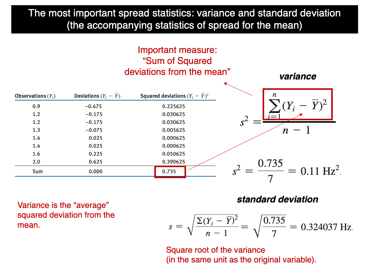
In simple terms, the variance is the sum of the squared differences (SS) between each value in the sample and the sample mean, divided by n-1. Many students encountering this for the first time often find it odd and wonder why SS isn’t divided by n instead of n-1. The reason lies in a correction called Bessel’s correction (https://en.wikipedia.org/wiki/Bessel%27s_correction), which is necessary to ensure the sample variance is an accurate (unbiased) estimate of the true population variance. Unbiased here means that, under random sampling, all possible sample variances from a population equal the population variance. In other words, in average, the sample variance will be equal to the true population variance and doesn’t tend to be greater or smaller. But that’s only when divided by n-1 as we will demonstrate (computationally) in this tutorial.
In Lecture 10, we saw that the sample variance is unbiased, but we used n-1 to calculate it for our small population - {1,2,3,4,5}
Let’s use a computational approach to demonstrate that when variance is calculated using n, it is biased, but when using n-1, it becomes unbiased.
The function var() in R calculates the sample variance, meaning that it divides by n - 1, not by n. In other words, it automatically applies the degrees-of-freedom correction so that the estimator is unbiased for the population variance.
It is also important to note that the function rnorm() generates data from a population distribution, and the argument sd refers to the population standard deviation.
quick.sample.data <- rnorm(n=100,mean=20,sd=2)
var(quick.sample.data)
var.byHand <- function(x) {sum((x-mean(x))^2/(length(x)-1))}
var.byHand(quick.sample.data)
Note that our function var.byHand() and the standard R function var gives exactly the same results. Notice also that, as such, we can use R to program our own functions.
Now let’s make a function in which the standard deviation is calculated using n in the denominator instead of n-1:
var.n <- function(x){sum((x-mean(x))^2)/(length(x))}
var.n(quick.sample.data)
Note that the value calculated using n is clearly smaller than the value calculated using n - 1. To understand this in the context of sampling estimation bias, let’s draw 100,000 samples from a normally distributed population with a sample size of n = 20, a population mean of 31, and a variance of 2 (which corresponds to a population standard deviation of 4).
lots.normal.samples.n20 <- replicate(100000, rnorm(n=20,mean=31,sd=2))For each sample, calculate the variance based on n-1 and n:
sample.var.regular <- apply(X=lots.normal.samples.n20,MARGIN=2,FUN=var)
sample.var.n.instead <- apply(X=lots.normal.samples.n20,MARGIN=2,FUN=var.n)
Let’s calculate the mean of all sample variances based on n-1 and n.
mean(sample.var.regular)
mean(sample.var.n.instead)
Note that the mean based on n-1 is extremely close to 4, i.e., the population parameter (not perfectly because we took 100000 samples instead of infinite). But the mean based on n is much smaller (should be around 3.8 or so), demonstrating that the correction to make the variance unbiased is necessary due to the issue of degrees of freedom that are covered in lecture 11.
That said, although the variance based on n-1 is not biased, the standard deviation based on n-1 is biased because the expected value (mean of all possible sample standard deviations) is not equal the true population standard deviation. Let’s see this issue in practice:
sample.sd.regular <- apply(X=lots.normal.samples.n20,MARGIN=2,FUN=sd)
mean(sample.sd.regular)
The population standard deviation is 2, but the average value calculated above is slightly smaller (~1.97), indicating a bias. This bias arises from the square root transformation of the variance as explained in Lecture 10.
The population standard deviation is 2, but the average value calculated above is slightly smaller (approximately 1.97), indicating a small bias. This bias arises from taking the square root of the variance, as discussed in Lecture 10. Because the square root is a nonlinear transformation, the expected value of the sample standard deviation does not exactly equal the population standard deviation.
Establishing a universally unbiased estimator for the standard deviation is challenging because the necessary correction depends on sample size. Although methods have been developed to address this (e.g., https://en.wikipedia.org/wiki/Unbiased_estimation_of_standard_deviation), the issue is not trivial.
Importantly, as we saw in Lecture 10, this bias is accounted for in statistical procedures such as the t-distribution. Rather than forcing the standard deviation itself to be perfectly unbiased, statistical theory incorporates its sampling behavior directly into the distribution used for inference.
In Lecture 10, we discussed how the t-distribution — which we use to construct confidence intervals — is built using the sample standard deviation. This means that the small bias present in the sample standard deviation is already incorporated into the t-distribution. In other words, the distribution we use for inference explicitly accounts for the fact that variability is being estimated from the sample.
It is also important to remember that this bias depends on sample size. When the sample size is small, the bias is more noticeable and the t-distribution is wider (reflecting greater uncertainty). As the sample size increases, the bias becomes negligible, and the t-distribution gradually approaches the normal distribution, becoming narrower.
For curiosity’s sake (you won’t be asked about this in exams), if the population is normally distributed, the sample standard deviation can be adjusted by dividing it by a constant derived from statistical theory. However, this correction is rarely applied in practice because it is unnecessary in most standard applications. As noted earlier, the theory behind this constant is mathematically advanced and goes beyond the scope of BIOL322. Still, being aware that such refinements exist can help you appreciate the depth and precision underlying statistical methodology.
mean(sample.sd.regular/0.986)Note that for n = 20, the correction constant is approximately 0.986. When each sample standard deviation is divided by this constant, the resulting value becomes an unbiased estimator of the true population standard deviation.
Observe that the mean of the corrected standard deviations (shown above) is now very close to 2. If we were able to take an infinite number of samples, the average of the corrected standard deviations would be exactly 2.
One important property of samples drawn from normally distributed populations is that the correlation between the sample means and their sample variances is zero. This occurs because, under normality, the sample mean and the sample variance are statistically independent. In other words, knowing the value of the sample mean provides no information about the value of the sample variance, and vice versa.
This independence is a special mathematical property of the normal distribution. Let’s demonstrate that from the generate data above. First, let’s calculate the mean of each sample since we haven’t done that yet:
sample.means <- apply(X=lots.normal.samples.n20,MARGIN=2,FUN=mean)Now, let’s plot the sample means and their variances:
plot(sample.means,sample.var.regular)Note that the cloud of points is oval rather than perfectly circular, yet their correlation is zero.
Correlation measures the strength and direction of a linear relationship between two variables. A correlation of zero means that there is no linear association; knowing the value of one variable does not help predict the value of the other in a linear way.
The cloud is not circular because the sampling distribution of the means is approximately normal and symmetric, whereas the sampling distribution of the variance is right-skewed and bounded below by zero. Even though the two quantities are uncorrelated, their different shapes and scales produce an oval pattern rather than a circle.
We will cover correlation later in the course, but we can calculate it as:
cor(sample.means,sample.var.regular)Note that the correlation is extremelly close to zero (could be a bit negative or positive, but in both cases almost zero)
Let’s plot the sampling distribution of the mean:
hist(sample.means)You can see that is highly symmetric. And the variance, as expected, highly asymetric:
hist(sample.var.regular)This guarantees mathematical independence between mean and variance.
Let’s assess the percentage coverage of confidence intervals. Remember that we set the population above with a true mean \(\mu\)=31.
First we need to find the t-value that will be used as multiplier:
n <- 20
t.crit <- qt(0.975, df = n - 1)
t.crit
We use 0.975 because we are constructing a two-sided 95% confidence interval. A 95% confidence interval leaves 5% of the probability outside the interval. Since the interval is two-sided, that 5% is split equally between the two tails of the t-distribution:
\(5\% = 2.5\% \text{ in the left/lower tail} + 2.5\% \text{ in the right/upper tail}\).
The function qt(p, df) gives the value t such that the probability to the left of that value is p.So when we write qt(0.975, df = n - 1), we are asking what t-value leaves 97.5% of the distribution to its left/lower tail? That value does not include the upper/right 2.5% tail. Because the t-distribution is symmetric, the corresponding lower cutoff is the negative of that value. That is why we use 0.975 to build a two-sided 95% confidence interval.
Now, let’s calculate all 100,000 confidence intervals; remember that we sampled 100,000 samples early one to generate the samples. ## 95% CI limits for each sample
ci.lower <- sample.means - t.crit * sample.sd.regular / sqrt(n)
ci.upper <- sample.means + t.crit * sample.sd.regular / sqrt(n)
Now, let’s calculate coverage, i.e., the percentage of intervals (out of 100,000 of them) that included the true population mean:
mu <- 31
covered <- (ci.lower <= mu) & (mu <= ci.upper)
Each expression inside parentheses is a logical condition: - (ci.lower <= mu) asks: Is the true mean greater than or equal to the lower bound? - (mu <= ci.upper) asks: Is the true mean less than or equal to the upper bound?
Each of those comparisons produces one logical value (TRUE or FALSE) for each sample. The symbol & means “and” in a logical (conditional) sense. It tells R: a value is TRUE only if both conditions are TRUE.
Let’s print the logical values for the first 10 confidence intervals:
covered[1:10]Now, let’s calculate coverage. This can be done using mean(covered). This works because when R calculates the mean of a logical vector, it automatically converts TRUE to 1 and FALSE to 0. Therefore, the mean of the logical values gives the proportion of intervals that contain the true population mean.
mean(covered)The coverage should be very close to ~0.95. If we had sampled infinite samples, it would had been exactly 0.95; but this simulation demonstrates how confidence intervals are expected to work, among other properties of sample estimators.
Plot only first 200 intervals; the ones that contain the true population mean are plotted in black and the ones that don’t contain are potted in green.
plot(1:200, sample.means[1:200],
     ylim = range(c(ci.lower[1:200], ci.upper[1:200], mu)),
     pch = 16, cex = 0.6,
     xlab = "Sample number",
     ylab = "Mean and 95% CI")

## Add confidence interval lines
segments(1:200, ci.lower[1:200],
         1:200, ci.upper[1:200],
         col = ifelse(covered[1:200], "black", "green"))

## Add true population mean
abline(h = mu, col = "red", lwd = 2)
When constructing confidence intervals from samples, we face a trade-off between long-run reliability and precision. If we choose a higher confidence level (for example, 99% instead of 95%), the interval becomes wider. This means that, in repeated sampling, a larger proportion of such intervals would contain the true population parameter. However, the estimate is less precise because the interval spans a broader range of values.
Conversely, if we choose a lower confidence level (for example, 90%), the interval becomes narrower and therefore more precise. But in repeated sampling, a smaller proportion of such intervals would contain the true value.
Thus, confidence intervals balance how often they succeed in the long run with how precise they are in any given sample.
How much does the validity of a confidence interval depend on the shape of the population distribution
With strongly asymmetric (or heavy-tailed) populations, the t-based confidence intervals for the mean may fail to achieve their nominal coverage. This is not simply because the standard deviation \(s\) is slightly biased, but because the t-procedure relies on the statistic \((\bar{x} - \mu)/(s/\sqrt{n})\) having an approximately t-shaped distribution; an approximation that can break down when the sampling distribution of the mean is far from normal (especially for small n). As sample size increases, the approximation typically improves, but for extreme skewness the convergence may not happen until sample size is extremely large.
Now load the data in R as follows:
humanGeneLengths <- as.matrix(read.csv("chap04e1HumanGeneLengths.csv"))
View(humanGeneLengths)
dim(humanGeneLengths)
The mean and variance of the population are:
mean.gene.pop <- mean(humanGeneLengths)
var.gene.pop <- var(humanGeneLengths)
Look at the distribution of the data and notice how asymmetric the distribution is:
hist(humanGeneLengths,xlim=c(0,20000),breaks=40,col='firebrick')We will use the gene data to demonstrate why the distribution of the population matters when working with sample estimators. Although we have the full population in this example, the principles we uncover are directly relevant to real-world settings, where the population is unknown and we must rely on samples.
Let’s begin by learning how to draw a sample from this population. To do this, we can use the sample() function in R. The key argument here is size, which specifies the sample size (in this example, n = 100 genes).
geneSample100 <- sample(humanGeneLengths, size = 100)
geneSample100
Now let’s assess the statistical properties of our sample estimators (the mean and the variance) by repeatedly sampling from the gene population. We will draw 100,000 samples, each of size n = 100, and then evaluate whether the sample mean and sample variance behave as unbiased estimators of the corresponding population values.
geneSample100 <- replicate(100000, sample(humanGeneLengths, size = 100))
dim(geneSample100)
Let’s calculate the mean and variance for each sample:
gene.sample.means <- apply(geneSample100,MARGIN=2,FUN=mean)
gene.sample.var <- apply(geneSample100,MARGIN=2,FUN=var)
And let’s compare the mean of all sample values with the population parameters:
c(mean(gene.sample.means),mean(humanGeneLengths))
c(mean(gene.sample.var),var(humanGeneLengths))
Let’s plot the sampling distribution of the mean:
hist(gene.sample.means)We can see that the distribution is more bell-shaped but still somewhat asymmetric.
Now, let’s plot the sample means against their sample variances:
plot(gene.sample.means,gene.sample.var)We can see that this patter is far different from what we observed early for a normally distributed population. And their correlation is quite different from zero and quite positive:
cor(gene.sample.means,gene.sample.var)You will notice that the two variables are no longer uncorrelated. This occurs because the sampling distribution of the sample means can exhibit some asymmetry, which induces a relationship between the mean and the variance across samples. Again, notice the asymmetry of the sampling distribution of the means.
hist(gene.sample.means)The sampling distribution of the variance is, in practice, almost always asymmetric. However, in this case it is noticeably more skewed than what we would observe for a normally distributed population with a similar sample size.
hist(gene.sample.var)Let’s create a sampling distribution for the same mean and variance for the gene population but based on a normally distributed population. And we will use the sample sample size of 100 observations:
sd.gene.pop <- sqrt(var.gene.pop)
lots.normal.samples.n100 <- replicate(100000, rnorm(n=100,mean=mean.gene.pop,sd=2))
sample.means.n100 <- apply(X=lots.normal.samples.n100,MARGIN=2,FUN=mean)
sample.var.n.100 <- apply(X=lots.normal.samples.n100,MARGIN=2,FUN=var)
Now let’s compare the two sampling distributions of the variance:
par(mfrow = c(1, 2))
hist(gene.sample.var,main="gene population",col = "lightgreen")
hist(sample.var.n.100,main="normal population",col = "lightblue")
You can see that the sampling distribution under normality is only slightly asymmetric, in contrast to the extremely skewed sampling distribution of the variance for the gene population.
When the population distribution is highly asymmetric, extreme values occur more often on one side. In this case, because the distribution of the population of gene lengths is right-skewed, extreme values will occur in the right side of the distribution. In repeated sampling, some samples will include one of these extreme observations while others will not. When a sample includes an extreme value, two things happen at the same time: the sample mean increases because the average is pulled toward the extreme value, and the sample variance increases dramatically because variance squares deviations from the mean. Since the same extreme observation simultaneously inflates both the mean and the variance, the two statistics tend to move together.
As a result, samples with larger means tend to also have larger variances, producing a positive association between them. This creates a nonzero correlation. The key point is that asymmetry introduces occasional large observations that affect both statistics in the same samples. As we saw earlier in this tutorial, under normality this does not occur in the same structured way, and the mean and variance remain independent. Under strong skewness, however, the shared influence of extreme values generates a correlation between the sample mean and the sample variance.
Because the t-distribution was derived under the assumption of normality — where the sample mean and the sample variance are independent — its use may be affected when the population distribution is strongly asymmetric or heavy-tailed.
Under normality, this independence ensures that the statistic:
\[\frac{\bar{x} - \mu}{s/\sqrt{n}}\] follows an exact t-distribution. However, when the population is highly skewed, extreme values can simultaneously influence both the mean and the variance, creating an association between them. Once this independence breaks down, the ratio above no longer follows a true t-distribution.
As a consequence, confidence intervals based on the t-distribution may not achieve their intended properties. For example, a 95% confidence interval may no longer contain the true mean 95% of the time. These distortions are typically more pronounced with small sample sizes and strong skewness, and they tend to diminish as sample size increases.
Let’s assess what this means for confidence intervals when sampling from the gene population. We will assess the coverage of t-based 95% CIs for the mean when population is the gene population. As above, we will sample size of n=100 and 100,000 repetitions.
Let’s generate a new set of samples from the gene population so we can practice the full workflow again and explicitly assess confidence-interval coverage. Of course, in real applications we usually do not know the true population, so we cannot evaluate coverage this directly. However, this exercise provides a clear demonstration of what can happen when key assumptions are not well met.
Sample genes from the population: using sample size n=100 and 100,000 replicates as before.
n <- 100
gene.samples <- replicate(100000, sample(humanGeneLengths, size = n, replace = TRUE))
Calculate the mean and standard deviation of each sample:
gene.means <- apply(gene.samples,2,mean)
gene.sds   <- apply(gene.samples,2,sd)
set the t critical value as we did before for assessing coverage from a normal distribution:
t.crit <- qt(0.975, df = n - 1)Calculate the confidence intervals:
gene.ci.lower <- gene.means - t.crit * gene.sds / sqrt(n)
gene.ci.upper <- gene.means + t.crit * gene.sds / sqrt(n)
Assess coverage as we did before for the normally distributed population.
mu.gene <- mean(humanGeneLengths)
gene.covered <- (gene.ci.lower <= mu.gene) & (mu.gene <= gene.ci.upper)
mean(gene.covered)
The coverage for n=100 genes is very close to 95% but a bit smaller.
Let’s assess coverage now with a smaller sample size, n=20.
n <- 20
gene.samples <- replicate(100000, sample(humanGeneLengths, size = n, replace = TRUE))
gene.means <- apply(gene.samples,2,mean)
gene.sds   <- apply(gene.samples,2,sd)
t.crit <- qt(0.975, df = n - 1)
gene.ci.lower <- gene.means - t.crit * gene.sds / sqrt(n)
gene.ci.upper <- gene.means + t.crit * gene.sds / sqrt(n)
mu.gene <- mean(humanGeneLengths)
gene.covered <- (gene.ci.lower <= mu.gene) & (mu.gene <= gene.ci.upper)
mean(gene.covered)
The coverage now should have been between 92% and 93%, which is lower than the 95% desired coverage.
Let’s plot the sampling distribution:
dev.off() # clean graph window. Often important when par was used before to plot multiple plots.
hist(gene.means)
It looks very asymmetric. Let’s plot the correlation between mean and variance:
gene.variances <- apply(gene.samples,2,var)
plot(gene.means,gene.variances)
cor(gene.means,gene.variances)
What do you observe?
Let’s assess coverage now with a much greater sample size, n=5000. This will take a minute or so.
n <- 5000
gene.samples <- replicate(100000, sample(humanGeneLengths, size = n, replace = TRUE))
gene.means <- apply(gene.samples,2,mean)
gene.sds   <- apply(gene.samples,2,sd)
t.crit <- qt(0.975, df = n - 1)
gene.ci.lower <- gene.means - t.crit * gene.sds / sqrt(n)
gene.ci.upper <- gene.means + t.crit * gene.sds / sqrt(n)
mu.gene <- mean(humanGeneLengths)
gene.covered <- (gene.ci.lower <= mu.gene) & (mu.gene <= gene.ci.upper)
mean(gene.covered)
Now, given the extremely large sample size, the coverage should be very close to 95%!
Let’s plot the sampling distribution:
hist(gene.means)It looks very symmetric. Let’s plot the correlation between mean and variance:
gene.variances <- apply(gene.samples,2,var)
plot(gene.means,gene.variances)
cor(gene.means,gene.variances)
What do you observe? Even though the confidence interval coverage is approximately correct, the sample mean and sample variance remain noticeably correlated. This indicates that the independence between mean and variance—an exact property under normality—does not hold here.
However, with this relatively large sample size, the t-based confidence intervals still perform well in terms of coverage. In other words, although the theoretical independence assumption is violated, the approximation underlying the t-distribution is sufficiently accurate at this sample size.
This exercise highlights an essential principle in statistical inference: the validity of confidence intervals depends not only on sample size, but also on the shape of the underlying population distribution.
However, when the population is strongly asymmetric, as in the gene length data, the situation changes. Extreme observations simultaneously influence both the sample mean and the sample variance, creating a correlation between them. This means that the exact independence property that holds under normality no longer applies, and strictly speaking, the statistic:
\[\frac{\bar{x} - \mu}{s/\sqrt{n}}\]
does not follow an exact t-distribution.
For small sample sizes, this breakdown can meaningfully affect inference, and t-based confidence intervals may fail to achieve their nominal coverage. However, as sample size increases, the Central Limit Theorem ensures that the sampling distribution of the mean becomes approximately normal, and the t-based procedure becomes increasingly accurate—even though the mean and variance remain correlated.
Central Limit Theorem (CLT): The Central Limit Theorem states that when we repeatedly take random samples of the same size from a population and calculate their sample means, the distribution of those sample means will become approximately normal as the sample size becomes large — regardless of the shape of the original population distribution. In simpler terms: Even if the population is skewed or irregularly shaped, the distribution of the sample mean will tend to look bell-shaped when the sample size is sufficiently large.
What we observed is both reassuring and instructive:
- For small samples (n = 20), coverage falls below 95% because the sampling distribution of the mean remains strongly asymmetric.
- For moderate samples (n = 100), coverage improves substantially.
- For very large samples (n = 5000), coverage is extremely close to 95%, even though the sample mean and variance are still correlated.
This demonstrates two important lessons: 1. The t-procedure relies on exact independence of mean and variance only for small-sample coverage exactness; it is remarkably robust in large samples. 2. Large sample sizes mitigate distortions through the Central Limit Theorem, even when theoretical assumptions such as independence between mean and variance do not strictly hold.
In practice, we rarely know the true population distribution. Therefore, we cannot evaluate coverage directly as we did here. But this simulation illustrates why assumptions matter, why sample size matters, and why many classical statistical procedures perform well in large samples—even when their theoretical conditions are only approximately satisfied.
Ultimately, confidence intervals reflect a balance between mathematical theory and practical robustness. Understanding when exact assumptions are critical and when asymptotic behavior provides protection is central to sound statistical thinking.
Transformations can often remove the bias in sample estimates
In previous sections, we saw that some sample estimators can be biased, especially when the population distribution is strongly asymmetric. This bias does not necessarily arise because the estimator is poorly defined, but because nonlinear relationships and skewed distributions affect how sample statistics behave across repeated sampling.
One common strategy to reduce or remove such bias is to transform the data. Transformations—such as taking the logarithm, square root, or other monotonic functions—can stabilize variance, reduce skewness, and make sampling distributions more symmetric. When the transformed data behave more like a normal distribution, sample estimators often perform better and statistical procedures based on normality become more reliable.
In this section, we will explore how transformations can change the behavior of sample estimators and improve inference.
The log-transformation of a sample is often used in biological and environmental sciences to reduce skewness and stabilize variability.
Generate samples and means:
n <- 20
gene.samples <- replicate(100000, sample(humanGeneLengths, size = n, replace = TRUE))
gene.means.log <- apply(log(gene.samples),2,mean)
gene.variances.log <- apply(log(gene.samples),2,var)
Note that the sampling distribution of the means is far more symmetric now than the original without log-transformation (for n=20).
hist(gene.means.log,main="log-transformed",col = "lightblue")Note that the sampling distribution of the variances is also a bit more symmetric than the original.
hist(gene.variances.log,main="log-transformed",col = "lightblue")The transformation still doesn’t remove the correlation between mean and variance but looks more oval as expexted for a normally distributed population:
plot(gene.means.log,gene.variances.log)
cor(gene.means.log,gene.variances.log)
Now let’s assess coverage; I’m redoing all the code here so that you can see all the steps together to assess coverage
# Log-transform population:
log.gene.pop <- log(humanGeneLengths)

# True mean on log-scale:
mu.log.gene <- mean(log.gene.pop)

# Sample size
n <- 20

# Generate samples from log-population
gene.samples <- replicate(100000,sample(log.gene.pop, size = n, replace = TRUE))

# Sample means and SDs (on log-scale)
gene.means <- apply(gene.samples, 2, mean)
gene.sds   <- apply(gene.samples, 2, sd)

# t critical value
t.crit <- qt(0.975, df = n - 1)

# Confidence intervals (log-scale)
gene.ci.lower <- gene.means - t.crit * gene.sds / sqrt(n)
gene.ci.upper <- gene.means + t.crit * gene.sds / sqrt(n)

# Coverage
gene.covered <- (gene.ci.lower <= mu.log.gene) & (mu.log.gene <= gene.ci.upper)

mean(gene.covered)
The coverage for n = 20 is now better and much closer to 95% than before. The square-root transformation tends to help for the same general reason: it reduces right-skewness and makes the sampling distribution of the mean more symmetric, which improves the accuracy of t-based confidence intervals on the transformed scale.
The important difference is the parameter we are estimating. After applying a transformation, the confidence interval no longer targets the original population mean. Instead, it estimates the mean of the transformed variable. Simply back-transforming the endpoints of the interval (for example, using exp() after a log transformation or squaring after a square-root transformation) does not, in general, produce a valid confidence interval for the arithmetic mean on the original scale.
If what we want scientifically is inference about the mean gene length on the original scale, we need a method designed for that target (for example, confidence intervals based on the mean with a different approximation, a bootstrap interval, or a model that fits the data distribution more directly).
Calculating confidence intervals on an empirical data
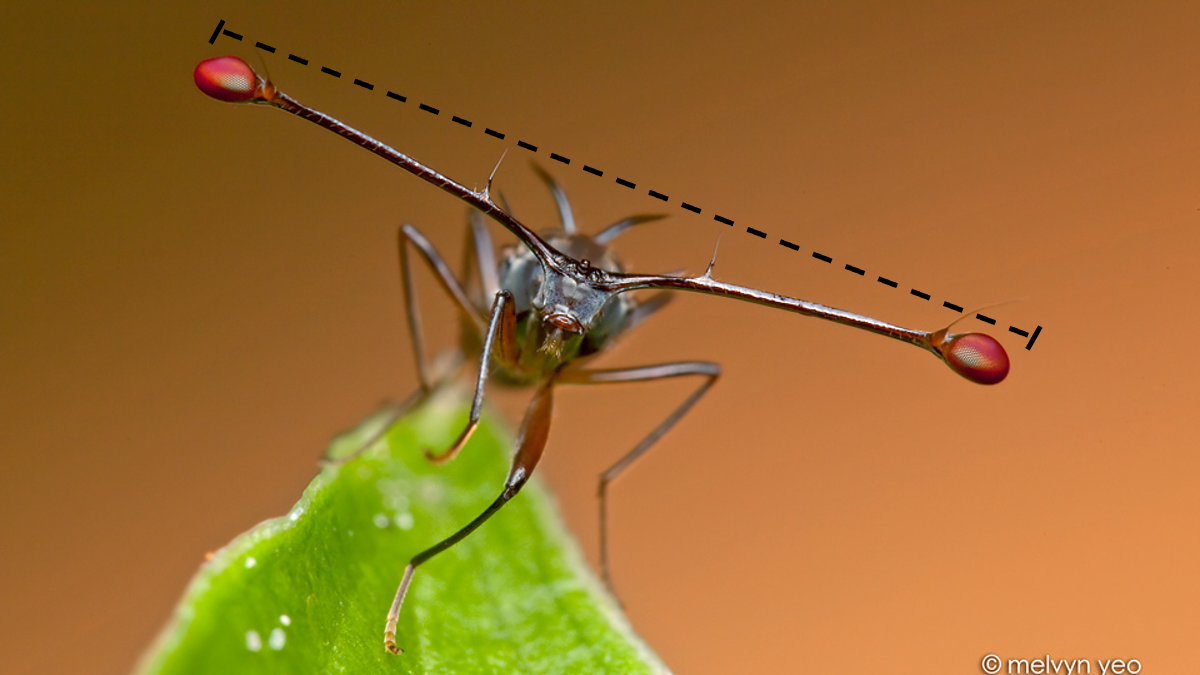
Let’s use a data set containing the span of the eyes (in millimeters) of nine male individuals of the stalk-eyed fly.
Download the stalk-eyed fly data file
Upload and inspect the data:
stalkie <- read.csv("chap11e2Stalkies.csv")
View(stalkie)
Let’s plot the histogram of the data. As you’ll see, the data appear relatively symmetric. This suggests that the distribution is approximately normal, allowing us to use the sample standard deviation as an estimate of the true population standard deviation. As we discussed in Lecture 10, confidence intervals are calculated using the t-distribution.
We’ll see later in the course how to assess the assumption of normality in a more rigorous way.
hist(stalkie$eyespan, col = "firebrick", las = 1,
    xlab = "Eye span (mm)", ylab = "Frequency", main = "")
Mean and standard deviation for the data:
mean(stalkie$eyespan)
sd(stalkie$eyespan)
Using the t-distribution, the 95% confidence interval for the population mean is:
t.test(stalkie$eyespan, conf.level = 0.95)$conf.intThe lower and upper limits of the interval appear in the first row of the output, i.e., the 95% confidence interval for the population mean is 8.471616 |—-| 9.083940
The 99% confidence interval is:
t.test(stalkie$eyespan, conf.level = 0.99)$conf.intExercise
Write code to show how a square-root transformation changes the sampling distribution of the mean when sampling from a strongly right-skewed population (Human Gene Lengths). Use a sample size of n = 20 and at least 100,000 repeated samples (with replacement).
Next, answer the question: Which mean is more likely to be close to its true population mean (parameter)—the mean on the original scale or the mean on the square-root scale? Use your sampling distributions to demonstrate your answer.
Focus solely on the sampling distributions of the mean—there’s no need to consider confidence intervals. Think (or write) a brief explanation of your answer, based on the code and the concepts covered in this tutorial.
Solution:
Because the gene-length population is strongly right-skewed, sample means on the original scale can be pulled upward by occasional extremely large values. This makes the sampling distribution of the mean more asymmetric and more spread out. Taking the square root reduces right-skewness, so the sampling distribution of the mean on the √-scale becomes more symmetric and tighter. Therefore, the square-root-scale sample mean is more likely to be close to its own true population mean (the mean of √gene length).
## ------------------------------------------------------------
## Code solution: Sampling distributions of the mean
## Human Gene Lengths: original scale vs square-root scale
## ------------------------------------------------------------

## Population (vector)
pop <- as.vector(humanGeneLengths)

## True population means (parameters) on each scale
mu_raw  <- mean(pop)
mu_sqrt <- mean(sqrt(pop))

## Simulation settings
n <- 20
n_sims <- 100000

## ------------------------------------------------------------
## Draw many samples and compute sample means
## ------------------------------------------------------------

## Sampling distribution of mean on original scale
samples_raw <- replicate(n_sims, sample(pop, size = n, replace = TRUE))
means_raw   <- apply(samples_raw, 2, mean)

## Sampling distribution of mean on square-root scale
samples_sqrt <- replicate(n_sims, sample(sqrt(pop), size = n, replace = TRUE))
means_sqrt   <- apply(samples_sqrt, 2, mean)

## Check centers (should be close to the true means)
c(mean(means_raw),  mu_raw)
c(mean(means_sqrt), mu_sqrt)