Tutorial 9: Two-sample t-tests
Statistical errors, significance level (alpha), statistical power, F-test for variance ratios, and paired and two-sample t-test
March 18 to 20, 2026
How the tutorials work
CRITICAL: Regular practice with R and RStudio, the statistical software used in BIOL 322 and introduced during tutorial sessions, and consistent engagement with tutorial exercises are essential for developing strong skills in Biostatistics. R tutorials will take place during the scheduled lab sessions.
EXERCISES: Each tutorial contains independent exercises and are not submitted for grading; however, students are strongly encouraged to complete them. Some tutorials include solutions at the end to support self-assessment and review. Other tutorials do not provide model answers because the exercises are procedural and can be easily self-assessed by checking that the code runs correctly and produces the expected type of output.
Your TAs
Section 0201: We 1:15pm-4:00pm, L-CC-213 - Sara Palestini (sarapalestini@gmail.com)
Section 0202: Th 1:15pm-4:00pm, L-CC-213 - Sara Palestini / Tristan Kolla
Section 0203: Fr 1:15pm-4:00pm, L-CC-203 - Snigdho Dutta (snigdhodeb29@gmail.com)
Section 0204: Fr 1:15pm-4:00pm, L-CC-213 - Tristan Kolla (tristan.kolla@mail.concordia.ca)
Understanding significance level (alpha), Type I error and Type II error.
The key takeaway from this initial part of the tutorial is: When making inferences from samples, we face an inherent trade-off: reducing the risk of one type of error (Type I, or false positives) necessarily increases the risk of the other (Type II, or false negatives).
To grasp the concept of the significance level (alpha level),vthe probability of committing a Type I error in a test, we’ll use the one-sample t-test (introduced in the last tutorial) to test the null hypothesis that human body temperature is 98.6°F (or 37°C, as commonly taught). Keep in mind that the principles we discuss here apply broadly to any statistical test!
Let’s assume the true population mean (which, in reality, we never know) is indeed \(\mu = 98.6^\circ\)F, and that the distribution of body temperatures in this population is normally distributed with a true standard deviation (sigma) of 2°F. Now, we’ll draw a sample from this population (25 individuals—the same sample size as in the body temperature study discussed in our lectures) and test whether we should reject the null hypothesis that the mean body temperature is 98.6°F.
This setup may seem redundant or obvious, as we’re sampling from a population with a known mean of 98.6°F to test the null hypothesis that the population mean is indeed 98.6°F. However, this “obviousness” (yes, that’s a real word!) can actually help clarify the principles underlying statistical tests.
Let’s start by taking a single sample from the statistical population:
sample.Temperature <- rnorm(n=25,mean=98.6,sd=2)
sample.Temperature
mean(sample.Temperature)
Although the sample is drawn from a population with a mean temperature of 98.6°F, the sample mean is unlikely to match this population value exactly—this difference is due to sampling error (not sampling bias, as the values were randomly selected; rnorm ensures random sampling) and is simply a result of chance. This should be second nature by now!
Next, we’ll test whether we should reject the null hypothesis based on our sample mean. Let’s quickly recap the null and alternative hypotheses for this scenario:
H0 (null hypothesis): the mean human body temperature is 98.6°F.
HA (alternative hypothesis): the mean human body temperature is different from 98.6°F.
Let’s conduct the one-sample t-test on your sample above:
t.test (sample.Temperature, mu=98.6)To extract just the p-value, simply:
t.test(sample.Temperature, mu=98.6)$p.valueMost likely, the p-value (assuming an alpha level of 0.05) was not significant (i.e., p-value > 0.05). But if it was, don’t be surprised. Here’s why this can happen: you may have committed a Type I error, where the test result was significant even though the null hypothesis was true. While making Type I errors (false positives, i.e., rejecting when you shouldn’t) isn’t ideal, they occur at the rate set by alpha (the significance level).
Accepting a low risk (e.g., 0.05 or 0.01) of Type I errors is what enables us to make inferences within the framework of statistical hypothesis testing.
A non-significant test result should come as no surprise, as the sample was drawn from a population with a true mean temperature of 98.6°F. Recall that in statistical hypothesis testing, we begin by assuming the null hypothesis is true (i.e., population mean = \(\mu\) = 98.6°F) and use the appropriate sampling distribution to account for sampling variation in the statistic of interest. In this case, the appropriate sampling distribution for sample means is the t-distribution.
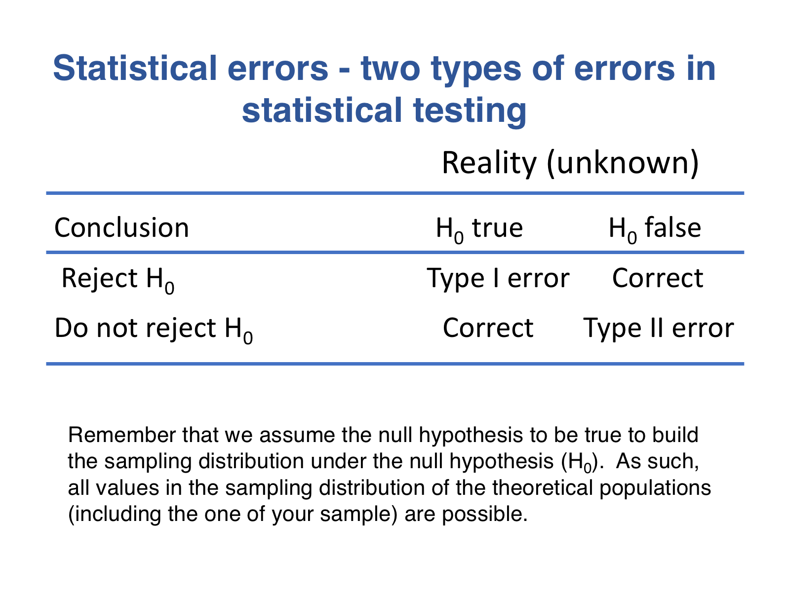
Let’s review first what type I and type II errors are:
Now, let’s draw a large number of samples from the population we specified earlier (population mean = 98.6°F) and test each sample against the null hypothesis:
number.samples <- 100000
samples.TempEqual.H0 <- replicate(number.samples,rnorm(n=25,mean=98.6,sd=2))
dim(samples.TempEqual.H0)
And for each sample, let’s run a t-test and extract its associated p-value; MARGIN is set below to 2 because we want to run the t-test in each column of the matrix where each sample was saved samples.Temp generated just above:
p.values <- apply(samples.TempEqual.H0,MARGIN=2,FUN=function(x) t.test(x, mu=98.6)$p.value)
length(p.values)
head(p.values)
The vector p.values holds all 100,000 p-values from t-tests conducted on each sample of 25 individuals, each drawn from a population with the same mean as the theoretical population assumed under the null hypothesis. Now, let’s calculate the percentage of tests (based on these samples) that produced significant p-values. What do you think this percentage will be?
alpha <- 0.05
n.rejections<-length(which(p.values<=alpha))/number.samples
n.rejections
n.rejections * 100 # percentage
As expected, the number of rejections closely aligns with the alpha level, \(\alpha = 0.05\) (in this case, it was 0.04996), meaning about 5% of tests on these samples were statistically significant. If we had set alpha to 0.01, then only about 1% of the samples would have been rejected. The slight deviation from exactly 0.05 is due to taking 100,000 samples rather than an infinite number from the statistical population of interest.
So, what does the significance level (\(\alpha\)) represent? It corresponds to the proportion of values considered significant when the null hypothesis is true. This is true here because we tested sample values from a population with the same mean as the theoretical population, meaning alpha is the probability of committing a Type I error. Thus, since the samples came from the same theoretical population assumed under the null hypothesis, the number of rejections aligns with alpha.
Now, consider what would happen if we set alpha to zero:
alpha <- 0.00
n.rejections<-length(which(p.values<=alpha))/number.samples
n.rejections
With alpha set to zero, we obviously don’t reject anything, as no p-value can be less than zero. This means we avoid committing any Type I errors. However, we would also never reject a null hypothesis, even in cases where it’s actually false, as we’ll discuss next.
This is the essence of the statistical hypothesis testing framework! We begin by identifying the appropriate sampling distribution under the assumption that the null hypothesis is true—here, the t-distribution. We then designate an alpha percentage of the t-values as significant, fully aware that these represent potential Type I errors. Why do we do this? Because we want to determine how unlikely it is to observe a sample mean (or a more extreme one) given the null hypothesis—in this case, using the t-distribution.
If we set \(\alpha = 0\), rejecting any null hypothesis becomes impossible. Let’s see this in action by taking a sample from a population with a higher mean temperature, say 99.8°F, while still testing against the original null hypothesis.
number.samples <- 100000
samples.TempDiferent.H0 <- replicate(number.samples,rnorm(n=25,mean=99.8,sd=2))
p.values <- apply(samples.TempDiferent.H0 ,MARGIN=2,FUN=function(x) t.test(x, mu=98.6)$p.value)
alpha <- 0.05
n.rejections<-length(which(p.values<=alpha))/number.samples
n.rejections
The number of rejections is around 0.82, meaning 82% of the samples were significant. This value represents the test’s statistical power (as discussed in our lectures). Statistical power is the probability of rejecting the null hypothesis when it is actually false. Here, we know the null hypothesis is false because the samples came from a population with a different mean than that assumed under the null hypothesis.
However, since we didn’t reject the null hypothesis in 100% of tests, we did commit some Type II errors. Specifically, 18% of the samples led to a non-rejection of the null hypothesis (1 - 0.82). As we covered in lecture, Type II error = 1 - statistical power.
But what happens with set an \(\alpha\) equal to zero:
alpha <- 0.00
n.rejections<-length(which(p.values<=alpha))/number.samples
n.rejections
Once again, we don’t reject any of the 100,000 tests, as no p-value can be less than zero. This means we’ve committed 100,000 Type II errors. To avoid this, we must accept some risk of rejecting the null hypothesis when it’s actually true—this is the risk of committing a Type I error, set by alpha. By doing so, we can reject the null hypothesis in cases where it’s false, thus reducing the number of Type II errors.
Remember, statistics are based on samples, and we never know the true value of a population parameter. Accepting a small chance of Type I errors (at a risk equal to alpha) allows us to avoid the greater risk of Type II errors. Recall the key point mentioned at the beginning of this tutorial?
When making inferences from samples, we face an inherent trade-off: reducing the risk of one type of error (Type I, or false positives) necessarily increases the risk of the other (Type II, or false negatives).
We hope that this now makes sense to you!
Paired comparison between two-sample means.
Are males with high testosterone incurring costs for their increased mating success in other areas?
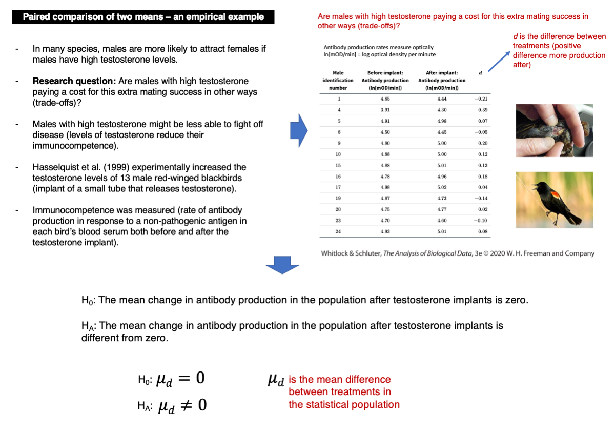
We will analyze data on individual differences in immunocompetence before and after increasing testosterone levels in red-winged blackbirds. Immunocompetence is measured as the logarithm of optical density, indicating antibody production per minute (ln[mOD/min]).
Download the testosterone data file
Now upload and inspect the data:
blackbird <- read.csv("chap12e2BlackbirdTestosterone.csv")
View(blackbird)
The original data differs significantly from what we would expect normally distributed data to look like (we’ll explore formal methods for assessing normality later in the course).
differences.d <- blackbird$afterImplant - blackbird$beforeImplant
hist(differences.d, col = "firebrick")
The data were log-transformed to make the data closer to normality. Calculate differences between after and before now:
differences.d <- blackbird$logAfterImplant - blackbird$logBeforeImplant
hist(differences.d, col = "firebrick")
Conduct the t-test:
t.test(differences.d)Given the p-value and assuming an alpha = 0.05, we should not reject the null hypothesis (p-value = 0.2277).
Testing for the difference between two independent sample means when the two samples can be assumed to have equal variances
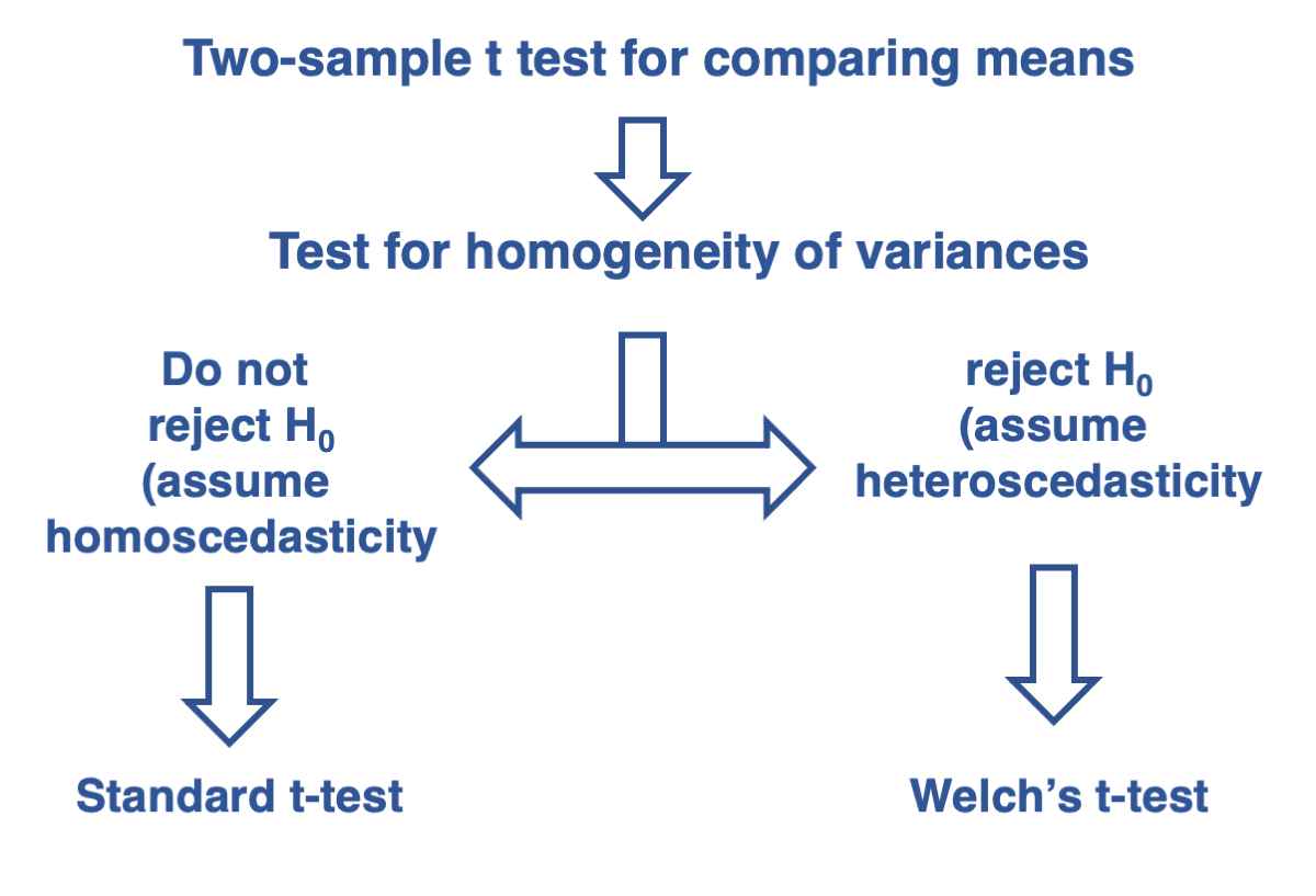
As we covered in Lecture 15, the t-test for two independent samples assumes that the populations from which the samples are drawn have equal variances. This assumption is essential for choosing the appropriate type of t-test. Remember our decision tree from the end of Lecture 15:
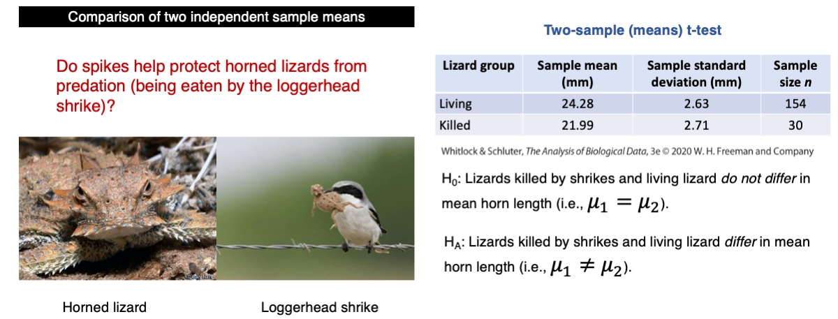
Do spikes help protect horned lizards from predation (being eaten)?
This is the problem we covered in Lecture 14 as an empirical example where the two-sample t-test was covered:
Download the horned lizard data file
Now upload and inspect the data:
lizard <- read.csv("chap12e3HornedLizards.csv")
View(lizard)
Let’s start by calculating the variances of each group of individuals, i.e., living and killed individuals:
living <- subset(lizard,Survival=="living")
length(living)
var(living$squamosalHornLength)
killed <- subset(lizard,Survival=="killed")
length(living)
var(killed$squamosalHornLength)
The variances for the living and killed individuals are 6.92 mm2 and 7.34 mm2, respectively. Although these values are close, we still need to test for homogeneity of variances.
var.test(squamosalHornLength ~ Survival, lizard, alternative = "two.sided")The null hypothesis should not be rejected (p-value = 0.7859).
Therefore, we can use the standard t-test for comparing two independent samples with the t.test function. Pay attention to the argument var.equal, which specifies that the t-test assumes equal variances between the two populations. This assumption was tested above, and the p-value indicates that it is reasonable to make this assumption.
t.test(squamosalHornLength ~ Survival, data = lizard, var.equal = TRUE)The p-value is 0.0000227 and we should reject the null hypothesis. The statistical conclusion is that lizards killed by shrikes and living lizard differ significantly in mean horn length.
Let’s calculate the mean of each sample:
mean(living$squamosalHornLength)
mean(killed$squamosalHornLength)
Because the sample mean of horn size of the living lizards is greater (24.28 mm) than the killed lizards (21.99 mm), we conclude that we have evidence that horn size is a protection against predation.
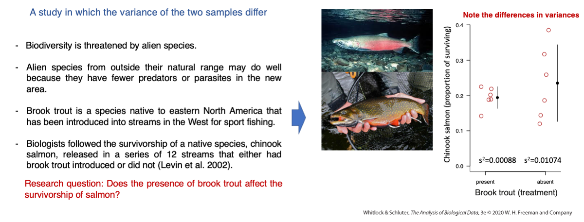
Testing for the difference between two independent sample means when the two samples CANNOT be assumed to have equal variances
Does the presence of brook trout affect the survivorship of salmon?
This is the problem we covered in lecture 15 as an empirical example where the two-sample Welch’s t-test was covered:
Now upload and inspect the data:
chinook <- read.csv("chap12e4ChinookWithBrookTrout.csv")
View(chinook)
names(chinook)
Let’s start by calculating the variances of each group of streams, i.e., with and without brook trout :
BrookPresent <- subset(chinook,troutTreatment=="present")
var(BrookPresent$proportionSurvived)
BrookAbsent <- subset(chinook,troutTreatment=="absent")
var(BrookAbsent$proportionSurvived)
The variance of proportion of chinook salmon individuals that survived in streams with brook trout is 0.00088 and without brook trout is 0.01074. If The variance ratio is indeed quite high:
var(BrookAbsent$proportionSurvived)/var(BrookPresent$proportionSurvived)The variance when brook trout was absent is 12.17 times greater than when brook trout was present.
This is a strong indication that one variance is much higher than the other, but are the two variances statistically different? The hypotheses are:
H0: The population variances of the proportion of chinook salmon surviving do not differ with and without brook trout. HA: The population variances of the proportion of chinook salmon surviving differ with and without brook trout.
var.test(proportionSurvived ~ troutTreatment , data = chinook)The p-value is 0.01589 and based on an alpha of 0.05, we reject the null hypothesis and we cannot assume that their variance are equal (homogenous or homoscedastic).
Since the null hypothesis of homogeneity of variances (homoscedasticity) is rejected, we should use the two-sample Welch’s t-test. This can be done by setting the argument var.equal to FALSE, which assumes that the two samples come from populations with different variances.
H0: The mean proportion of chinook surviving is the same in streams with and without brook trout.
HA: The mean proportion of chinook surviving differs in streams with and without brook trout.
t.test(proportionSurvived ~ troutTreatment , data = chinook,var.equal = FALSE)Exercise
Exercise 1 — Interpreting the error trade-off
You conduct a one-sample t-test with \(\alpha\) = 0.01 instead of \(\alpha\) = 0.05.
Explain how this change affects:
1.  The probability of committing a Type I error
2.  The probability of committing a Type II error
3.  The statistical power of the test
Exercise 2 — Interpreting simulation results
You run the simulation described in the tutorial with \(\alpha\) = 0.05 and obtain a rejection rate of 0.048.
Question: Why is the rejection rate not exactly 0.05, and what does this result represent conceptually?
Exercise 3 — Paired vs independent design
A researcher measures immune response in birds before and after a hormone treatment.
Question: Explain why a paired t-test is more appropriate than a two-sample independent t-test in this case, and describe what would be lost if the data were analyzed as independent samples.
Exercise 4 — Choosing the correct t-test
You compare two groups and obtain the following:
- Variance test p-value = 0.012
- Two-sample t-test performed with var.equal = TRUE
Question: Is this analysis appropriate? If not, explain what should have been done and why.
Exercise 5 — Interpreting power and Type II error
In a simulation where the true mean differs from the null hypothesis, you obtain a rejection rate of 0.82.
Question: 1. What does this value represent? 2. What is the probability of committing a Type II error? 3. Explain why this error still occurs even though the null hypothesis is false.
Answers
Exercise 1: Reducing \(\alpha\) from 0.05 to 0.01 decreases the probability of committing a Type I error because fewer outcomes are considered statistically significant. However, this stricter criterion makes it harder to reject the null hypothesis, which increases the probability of committing a Type II error. As a result, statistical power decreases because the test becomes less likely to detect a true effect when it exists.
Exercise 2: The rejection rate is not exactly 0.05 because the simulation uses a finite number of samples (e.g., 100,000) rather than an infinite number. Small deviations are expected due to random sampling variation. Conceptually, this rejection rate represents the empirical probability of committing a Type I error, which approximates \(\alpha\) when the null hypothesis is true.
Exercise 3: A paired t-test is appropriate because the measurements before and after treatment are taken on the same individuals, meaning the observations are not independent. The paired test accounts for within-individual variation by analyzing the differences directly. If analyzed as independent samples, this pairing structure would be ignored, increasing variability and reducing statistical power, making it harder to detect a true effect.
Exercise 4: Answer: This analysis is not appropriate. A variance test p-value of 0.012 indicates that the assumption of equal variances should be rejected (at \(\alpha\) = 0.05). Therefore, the standard two-sample t-test assuming equal variances should not be used. Instead, Welch’s t-test (var.equal = FALSE) should be applied because it does not assume equal variances and provides a more reliable inference under heteroscedasticity.
Exercise 5: Answer: The value 0.82 represents the statistical power of the test, which is the probability of correctly rejecting the null hypothesis when it is false. The probability of committing a Type II error is 1 - 0.82 = 0.18. This error occurs because sampling variability can still produce sample means close to the null value, leading to non-significant results even when the true population mean differs.