Lecture 18: post-hoc ANOVA

November 15th, 2022 (10th week of classes)

---

post-hoc ANOVA analysis

Once the null hypothesis of an ANOVA is rejected, we favor the alternative hypothesis in which “at least two samples come from different statistical populations with different means”. That said, ANOVA doesn’t allow us to determine which pairs of means are significantly different from one another. This is an important step to interpret further the outcome of research studies. This analysis is called post-hoc, i.e., after ANOVA was conducted. We also cover the important tests to assess that the assumption of homoscedasticity holds so that we can conduct an ANOVA on the data.

---

Lecture

Slides:

Download lecture: 3 slides per page and outline

Download lecture: 1 slide per page

Video:

---

Supplement to the lecture (demonstration of principles involving family-wise Type I error using code)

There is no need to study the code below but it will allow to understand further the issues discussed in this lecture.

We saw ttat if we set an alpha of 0.05, i.e., acceptance area of 95% (0.95), then the chance of finding at least one significant test when you should not (i.e., committing one Type I error or a false positive error) out of 24 tests is:

\[1-0.95^{24}=0.708011\]

The code below reproduces the plot on how the probability of at least one type I error changes as a function of number of tests. It turns out that to achieve a probability of 100% we need at least 328 tests.

n.tests <- 1:328
prob.atLeast1.TypeIerror <- 1 - 0.95^n.tests
prob.atLeast1.TypeIerror[325:328]

## [1] 0.9999999 0.9999999 0.9999999 1.0000000

plot(n.tests,prob.atLeast1.TypeIerror,pch=16,col="firebrick",
     cex=0.3, xlab="number of tests",ylab="prob. of at least one type I error")

The code below then generates 328 two-sample t tests when all tests are based on sampling from the same population, i.e., any significance would be true false positives (i.e., type I errors). 328 two-sample t tests are repeated 1000 times. Each time, the number of significant p-values are counted and recorded in the vector number.TypeIerrors.

number.samples <- 328
groups <- c(rep(1,15),rep(2,15))
number.TypeIerrors <- c()
for (i in 1:1000){
  samples.H0.True <- replicate(number.samples,rnorm(n=30,mean=10,sd=3))
  p.values <- apply(samples.H0.True,MARGIN=2,FUN=function(x) t.test(x~groups,var.equal = TRUE)$p.value)
  number.TypeIerrors[i] <- length(which(p.values <= 0.05))
}

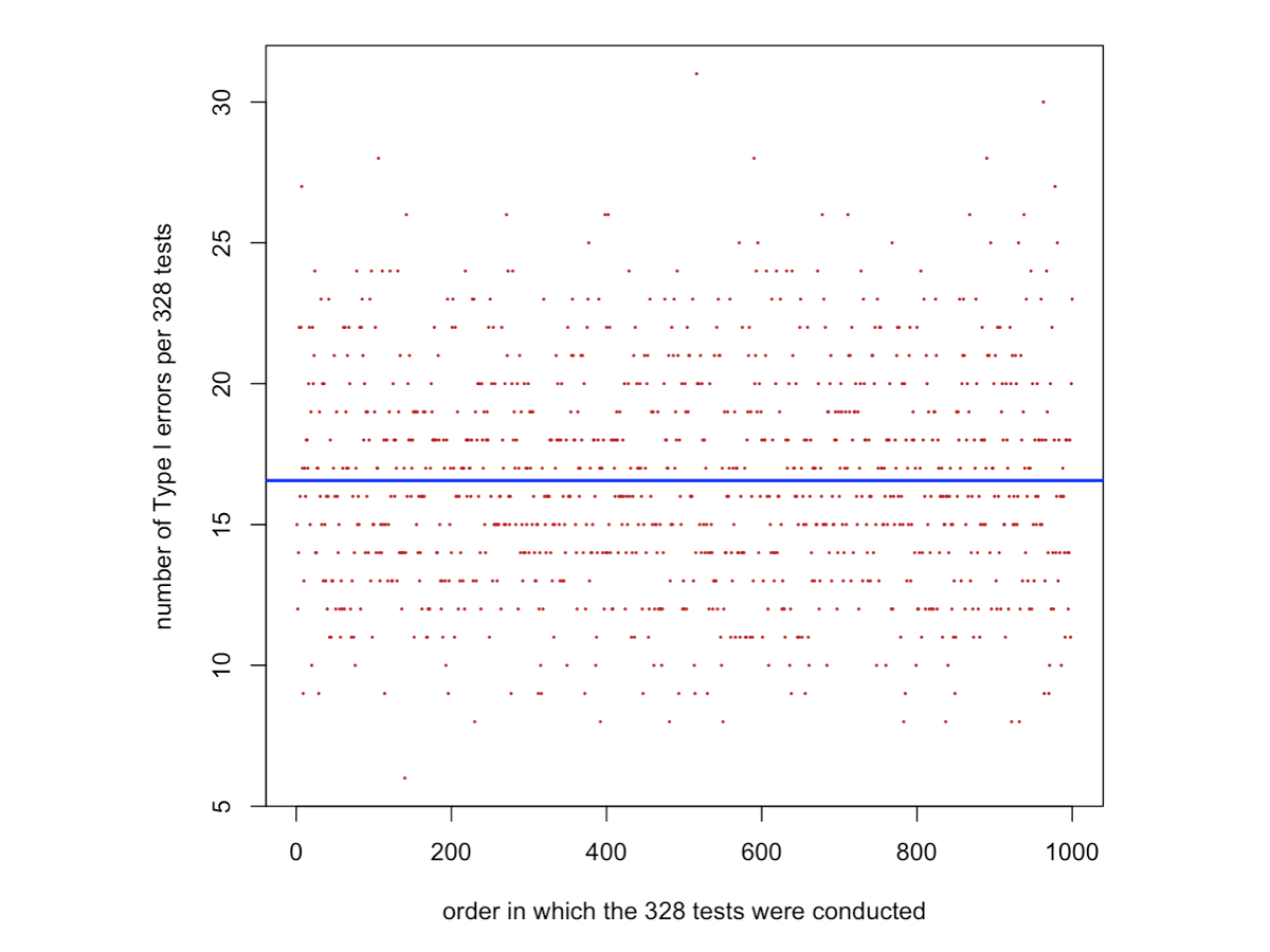
Code for plotting the number of type I errors per 328 two-sample t-tests in the order they were performed. The blue line shows the average number of type I error rates estimated from the data, which is given by mean(number.TypeIerrors). This value should be extremely similar to 16.4, which is the expected number of values given by 0.05 x 328. In order words 5% of tests are expected in average to be siginificant when they should not (i.e., a product of multiple Type I errors, called the family-wise type I error as discussed in the lecture). mean(number.TypeIerrors) is not exactly 0.05 x 328 (the true average value) because we calculated mean(number.TypeIerrors) based on 1000 times 328 tests. They would be equal if we had run infinite times 328 tests.

plot(1:1000,number.TypeIerrors,pch=16,col="firebrick",cex=0.3,xlab="order in which the 328 tests were conducted",ylab="number of Type I errors per 328 tests")
abline(h=mean(number.TypeIerrors),col="blue",lwd=2)
expected.avg.typeIerror <- 0.05*328
mean(number.TypeIerrors)