Tutorial 9: Two-sample t-tests
Statistical errors, significance level (alpha), statistical power, F-test for variance ratios, and paired and two-sample t-test
Week of November 7, 2022
(9th week of classes)
How the tutorials work
The DEADLINE for your report is always at the end of the tutorial.
The INSTRUCTIONS for this report is found at the end of the tutorial.
Students may be able after a while to complete their reports without attending the synchronous lab/tutorial sessions. That said, we highly recommend that you attend the tutorials as your TA is not responsible for assisting you with lab reports outside of the lab synchronous sections.
The REPORT INSTRUCTIONS (what you need to do to get the marks for this report) is found at the end of this tutorial.
Your TAs
Section 101 (Wednesday): 10:15-13:00 - John Williams (j.p.w@outlook.com)
Section 102 (Wednesday): 13:15-16:00 - Hammed Akande (hammed.akande@mail.mcgill.ca)
Section 103 (Friday): 10:15-13:00 - Michael Paulauskas (michael.paulauskas@mail.mcgill.ca)
Section 104 (Friday): 13:15-16:00 - Alexandra Engler (alexandra.engler@hotmail.fr)
Understanding significance level (alpha), Type I error and Type II error.
The biggest realization from this first part of the tutorial should be - There is a small statistical price to pay when inferring from samples: we need to accept a small risk of committing one sort of error (Type I or false positives) to avoid a bigger risk of committing another sort of error (type II or false negatives).
To understand the significance level (alpha level), which is the risk (probability) of committing a type I error of a test, we will use the one-sample t-test (seen in the last tutorial) for testing the null hypothesis that the human body temperature is 98.6°F (or 37°C, as taught in schools). Note, however, that the concepts discussed here apply to any statistical test!
Let’s assume that the true population value (which we never know in reality) is indeed \(\mu\)=98.6°F. Now, let’s assume that the distribution of temperatures in the true human population is normally distributed with a true standard deviation (sigma) of 2°F. Next, we will take a sample from this population (25 individuals; the same number of individuals as in the human body temperature study seen in our lectures) and test whether we should reject or not the null hypothesis that the true mean temperature is 98.6°F. This seems redundant and obvious because you are sampling from a population with a true mean of 98.6°F and testing the null hypothesis that true population mean is 98.6°F. This “obviousness” (yes, this word exists), however, should help you further understand the principles involved in a statistical test.
Let’s start by taking a single sample from the statistical population:
sample.Temperature <- rnorm(n=25,mean=98.6,sd=2)
sample.Temperature
mean(sample.Temperature)
Although the sample came from a population with a mean temperature of 98.6°F, the mean of the sample is not exactly equal to the population value, i.e., there is sampling error (not sampling bias as values were sampled randomly; rnorm assures random sampling) due to chance! No big surprise, this should be first nature to you by now.
Now let’s test whether we should reject or not the null hypothesis based on our sample value. Let’s recap the null and alternative hypotheses involved here:
H0 (null hypothesis): the mean human body temperature is 98.6°F.
HA (alternative hypothesis): the mean human body temperature is different from 98.6°F.
Let’s conduct the one-sample t-test on your sample above:
t.test (sample.Temperature, mu=98.6)To extract just the p-value, simply:
t.test(sample.Temperature, mu=98.6)$p.valueMost likely the p-value (say assuming an alpha=0.05) was not significant (i.e., p-value should be greater than alpha=0.05). But if it was, don’t be surprised. The following will help you understand why this may happen, i.e., you committed a Type I error in which the test outcome was significant even though the null hypothesis was true. Although committing Type I errors (false positives, i.e., reject when you should not) is not desirable, it will happen with the percentage we set for alpha (i.e.,the significance level). Committing a type I error with a low risk (probability; say of 0.05 or 0.01) is what allows us to make statistical inferences using the statistical hypothesis testing framework.
A non-significant test should come as no surprise. This is because the sample was taken from a population that has a true mean temperature equal to 98.6°F. Remember that the way we test a statistical hypothesis is based on first assuming that the null hypothesis is true (population mean = \(\mu\) = 98.6°F) and use the appropriate sampling distribution that describes sampling variation for the statistic of interest. Here, the appropriate sampling distribution of sample means is the t-distribution.
Let’s review first what type I and type II errors are:
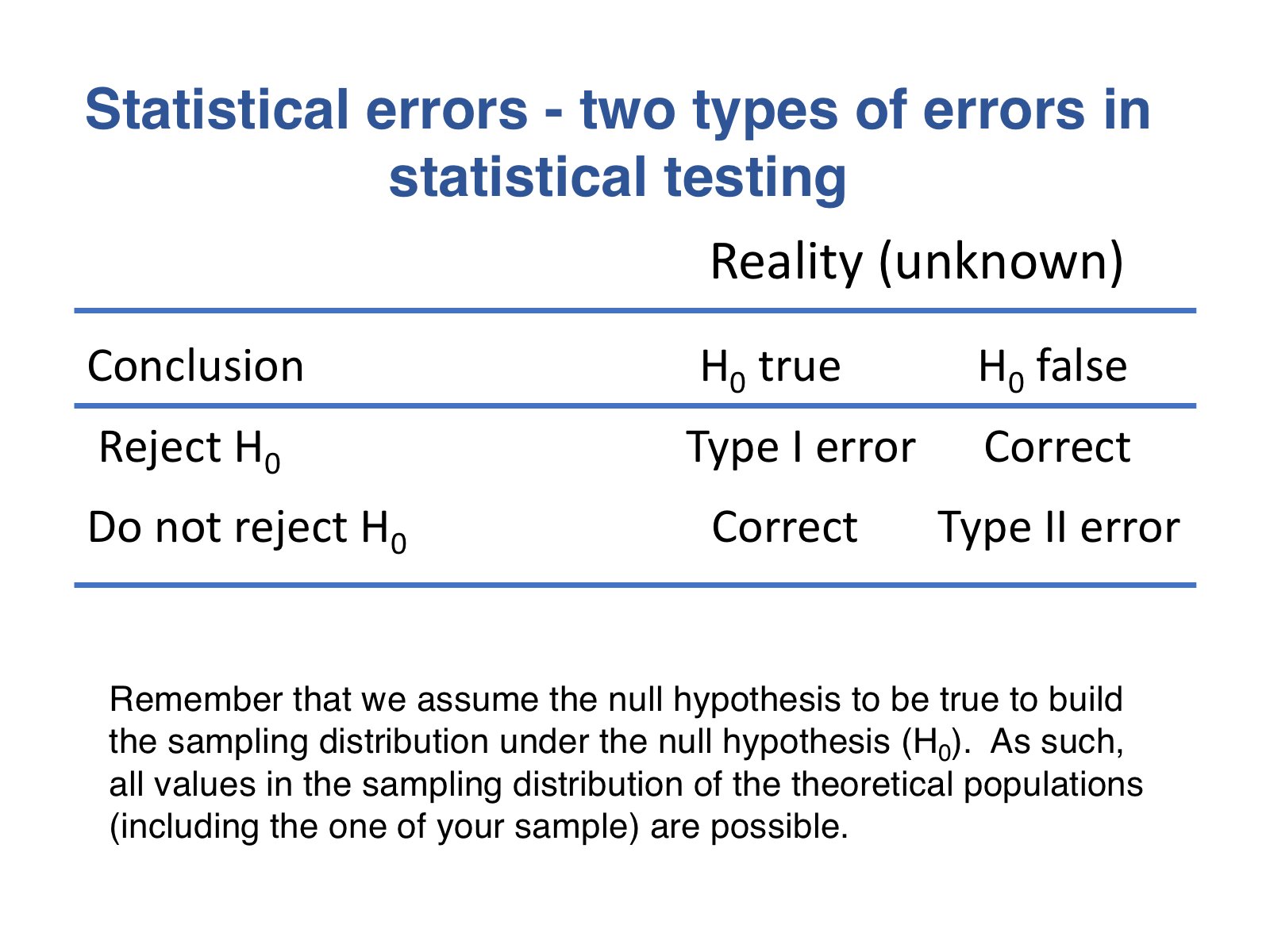
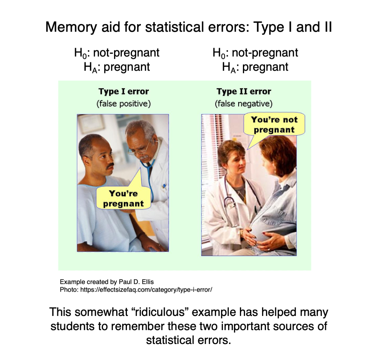
This memory aid (which is not about samples) may help you to associate better type I and type II errors to false positives and false negatives, respectively:
Let’s now take a large number of samples from the population we set earlier (i.e., population mean = 98.6°F) and test each of them against the null hypothesis:
number.samples <- 100000
samples.TempEqual.H0 <- replicate(number.samples,rnorm(n=25,mean=98.6,sd=2))
dim(samples.TempEqual.H0)
And for each sample, let’s run a t-test and extract its associated p-value; MARGIN is set below to 2 because we want to run the t-test in each column of the matrix where each sample was saved samples.Temp generated just above:
p.values <- apply(samples.TempEqual.H0,MARGIN=2,FUN=function(x) t.test(x, mu=98.6)$p.value)
length(p.values)
head(p.values)
The vector p.values contains all the 100000 p-values for the t-test on each sample of 25 individuals that were sampled from a population with exactly the same mean value of the theoretical population we assumed for the null hypothesis in the t-test. So, let’s calculate what is the percentage of tests (i.e., based on the samples) for which their p-values were significant. What do you think that value will be?
alpha <- 0.05
n.rejections<-length(which(p.values<=alpha))/number.samples
n.rejections
n.rejections * 100 # percentage
Well, the number of rejections is pretty close to the alpha level \(\alpha\) = 0.05 (in my case it was 0.04996), i.e., 5% of the tests on the samples were statistically significant. If alpha had been set as 0.01, then only about 1% of the samples would had been rejected. The reason that is not perfectly 0.05 is because we took 100000 samples and not an infinite number of samples from the statistical population of interest! What does the significance level (\(\alpha\)) match to? It is equal to the number of values that are considered as significant when the null hypothesis is true; it’s true because we tested sample values from a population that has the same mean as the theoretical population: so alpha is the probability of committing a Type I error! So, obviously, because the samples were taken from the same theoretical population as the one assumed under the null hypothesis, then the number of rejections has to be alpha. What happens if we set alpha equal to zero:
alpha <- 0.00
n.rejections<-length(which(p.values<=alpha))/number.samples
n.rejections
Well, we obviously don’t reject anything because no p-value can be smaller than zero. As such, we don’t commit a type I error. However, we won’t ever reject any null hypothesis either, even in the cases where they are not true as we discuss next.
This is the statistical hypothesis testing framework!!! We start by identifying the appropriate sampling distribution assuming the null hypothesis as true; here the t-distribution. We then consider an alpha percent of the t-values to be significant even knowing that they will represent a Type I error. Why do we do that? Because we are interested in determining how unlikely a sample mean or a more extreme sample mean is given the null hypothesis (i.e., the t-distribution in the case here). If we set \(\alpha\) = 0, then it becomes impossible to reject any null hypothesis. Let’s see that in practice by taking a sample from a statistical population with a greater temperature, say 99.8°F, but still testing against the original null hypothesis.
number.samples <- 100000
samples.TempDiferent.H0 <- replicate(number.samples,rnorm(n=25,mean=99.8,sd=2))
p.values <- apply(samples.TempDiferent.H0 ,MARGIN=2,FUN=function(x) t.test(x, mu=98.6)$p.value)
alpha <- 0.05
n.rejections<-length(which(p.values<=alpha))/number.samples
n.rejections
The number of rejections will be around 0.82, i.e., 82% of the samples were significant. By the way, this is what the power of the test is (as seen in our lectures). Statistical power is the probability of rejecting the null hypothesis when the null hypothesis is in reality false. We knew that it was false because (i.e., the samples were taken from a population with a different mean than the one assumed under the null hypothesis). Note, however, that because we were not able to reject 100% of the tests, we committed some Type II errors, i.e., 18% of the samplea above led to a non-rejection of the null hypothesis (1-0.82). As we saw in our lecture, Type II error = 1 - statistical power.
But what happens with set an \(\alpha\) equal to zero:
alpha <- 0.00
n.rejections<-length(which(p.values<=alpha))/number.samples
n.rejections
Again, we obviously don’t reject any of the 100000 tests because no p-value can be smaller than zero. So, here we committed 100000 type II errors.
As such, we need to accept some risk to reject the null hypothesis when we should not, i.e., commit a Type I error (this risk = alpha) so that we can reject many more, i.e., not commit Type II errors. Remember that statistics are based on samples. Because we never know the true value of the parameter of the statistical population, we need to commit a few Type I errors (at a risk equal to alpha) to avoid the larger risk of committing type II errors! Do you remember the first thing that was said in the beginning of this tutorial?
There is a small statistical price to pay when inferring from samples: we need to accept a small risk of committing one sort of error [i.e., type I error] to avoid a bigger risk of committing another sort of error [i.e., type II error].
I hope you now understand what that means!
Paired comparison between two-sample means.
Are males with high testosterone paying a cost for this extra mating success in other ways?
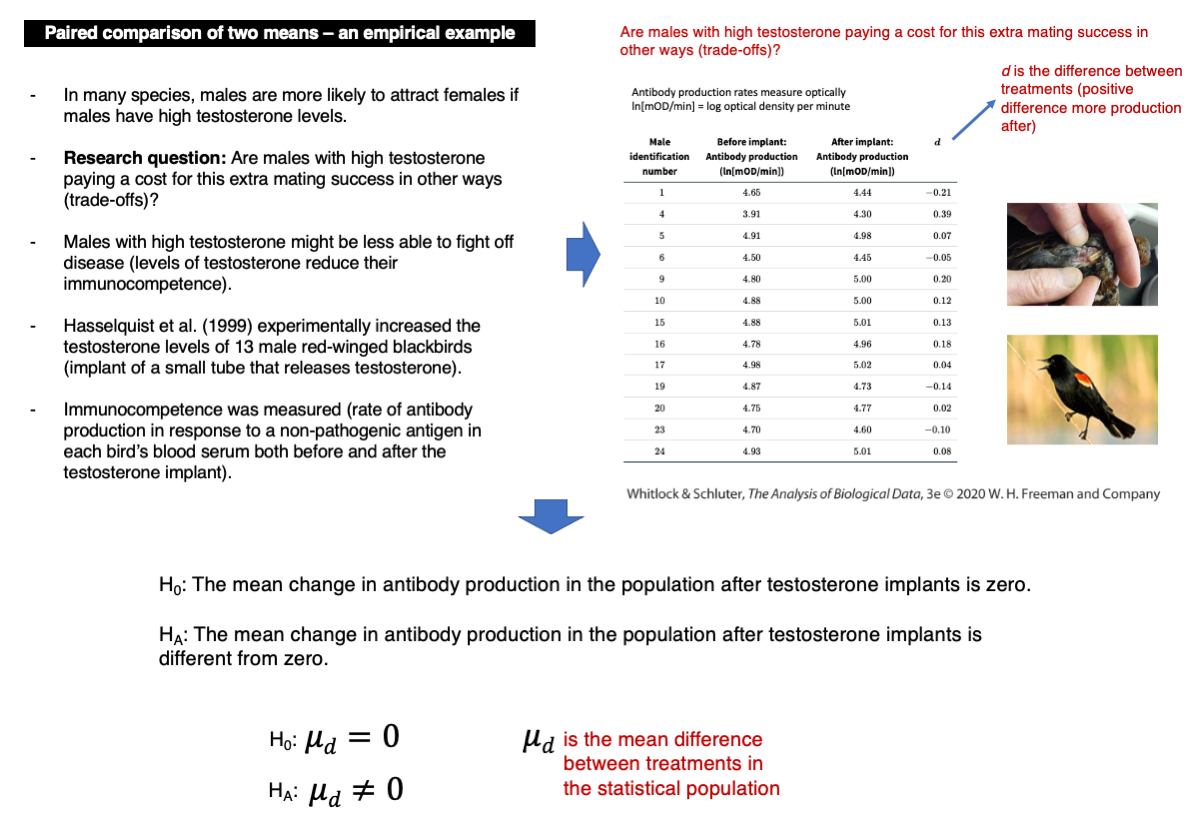
We will use the data on individual differences in immunocompetence before and after increasing the testosterone levels of red-winged blackbirds. Immunocompetence was measured as the log of optical measures of antibody production per minute (ln[mOD/min]).
Download the testosterone data file
Now upload and inspect the data:
blackbird <- read.csv("chap12e2BlackbirdTestosterone.csv")
View(blackbird)
The original data is quite different from what normally distributed data should look like (we will see more formal ways to assess normality later in the course).
differences.d <- blackbird$afterImplant - blackbird$beforeImplant
hist(differences.d, col = "firebrick")
The data were log-transformed to make the data closer to normality. Calculate differences between after and before now:
differences.d <- blackbird$logAfterImplant - blackbird$logBeforeImplant
hist(differences.d, col = "firebrick")
Conduct the t-test:
t.test(differences.d)Given the p-value and assuming an alpha = 0.05, we should not reject the null hypothesis (p-value = 0.2277).
Testing for the difference between two independent sample means when the two samples can be assumed to have equal variances
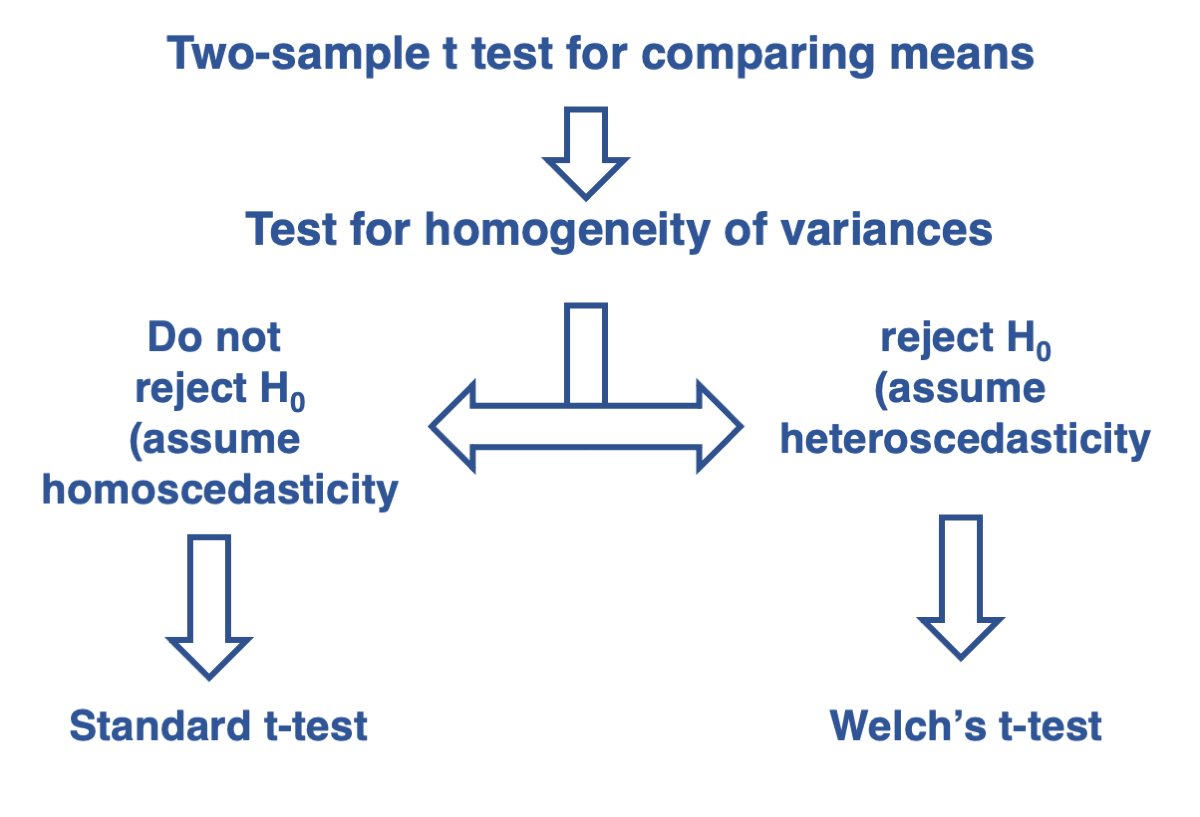
As covered in lecture 15, the t-test for two independent samples assume that the variances of the populations where the samples came from have equal variances. This is important to select the appropriate type of t-test to use. Remember our decision tree at the end of lecture 15:
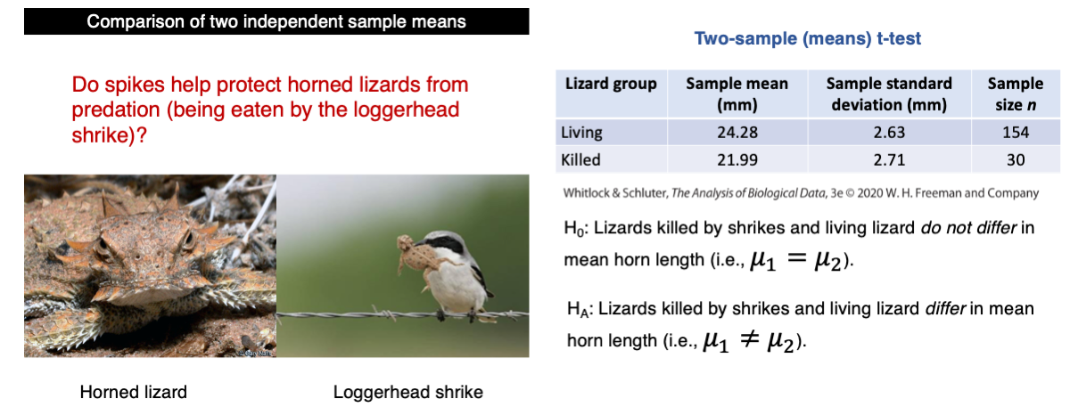
Do spikes help protect horned lizards from predation (being eaten)?
This is the problem we covered in Lecture 14 as an empirical example where the two-sample t-test was covered:
Download the horned lizard data file
Now upload and inspect the data:
lizard <- read.csv("chap12e3HornedLizards.csv")
View(lizard)
Let’s start by calculating the variances of each group of individuals, i.e., living and killed individuals:
living <- subset(lizard,Survival=="living")
length(living)
var(living$squamosalHornLength)
killed <- subset(lizard,Survival=="killed")
length(living)
var(killed$squamosalHornLength)
The variance for the living and killed individuals are 6.92 mm2 and 7.34 mm2, respectively. They are not that different, but we need to test for the homogeneity of their variances.
var.test(squamosalHornLength ~ Survival, lizard, alternative = "two.sided")The null hypothesis should not be rejected (p-value = 0.7859).
As such, we can use the standard t-test for comparing two independent samples using the function t.test. Note the argument var.equal. This argument sets the t-test for the case in which we can assume that the two samples come from populations that have equal variances. This assumption was tested above, and the p-value suggests that this assumption is warranted.
t.test(squamosalHornLength ~ Survival, data = lizard, var.equal = TRUE)The p-value is 0.0000227 and we should reject the null hypothesis. The statistical conclusion is that lizards killed by shrikes and living lizard differ significantly in mean horn length.
Let’s calculate the mean of each sample:
mean(living$squamosalHornLength)
mean(killed$squamosalHornLength)
Because the sample mean of horn size of the living lizards is greater (24.28 mm) than the killed lizards (21.99 mm), we conclude that we have evidence that horn size is a protection against predation.
Testing for the difference between two independent sample means when the two samples CANNOT be assumed to have equal variances
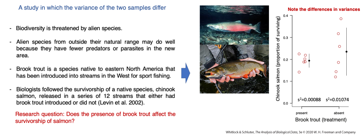
Does the presence of brook trout affect the survivorship of salmon?
This is the problem we covered in lecture 15 as an empirical example where the two-sample Welch’s t-test was covered:
Now upload and inspect the data:
chinook <- read.csv("chap12e4ChinookWithBrookTrout.csv")
View(chinook)
names(chinook)
Let’s start by calculating the variances of each group of streams, i.e., with and without brook trout :
BrookPresent <- subset(chinook,troutTreatment=="present")
var(BrookPresent$proportionSurvived)
BrookAbsent <- subset(chinook,troutTreatment=="absent")
var(BrookAbsent$proportionSurvived)
The variance of proportion of chinook salmon individuals that survived in streams with brook trout is 0.00088 and without brook trout is 0.01074. If The variance ratio is indeed quite high:
var(BrookAbsent$proportionSurvived)/var(BrookPresent$proportionSurvived)The variance when brook trout was absent is 12.17 times greater than when brook trout was present.
This is a strong indication that one variance is much higher than the other, but are the two variances statistically different? The hypotheses are:
H0: The population variances of the proportion of chinook salmon surviving do not differ with and without brook trout. HA: The population variances of the proportion of chinook salmon surviving differ with and without brook trout.
var.test(proportionSurvived ~ troutTreatment , data = chinook)The p-value is 0.01589 and based on an alpha of 0.05, we reject the null hypothesis and we cannot assume that their variance are equal (homogenous or homoscedastic).
Given that the null hypothesis of homogeneity of variances (homoscedasticity) is rejected, we should use the two-sample Welch’s t-test. The Welch’s t-test can be conducted simply by setting the argument var.equal below as FALSE, i.e., assume that the two samples come from statistical populations that have different variances.
H0: The mean proportion of chinook surviving is the same in streams with and without brook trout.
HA: The mean proportion of chinook surviving differs in streams with and without brook trout.
t.test(proportionSurvived ~ troutTreatment , data = chinook,var.equal = FALSE)Report instructions
By now, you should be used to the fact that many tutorial report problems can be solved by copying and pasting code covered in the tutorial, but making the appropriate adjustments to solve the problem at hands. This is a way to practice and help you understand the concepts covered in the tutorial.
Part 1: Based on a significance level (alpha) equal to 0.05, what is the statistical conclusion for the test you just performed (i.e., t-test for the chinook salmon problem)? What is the scientific conclusion?
Part 2: Based on the simulations in the first part of the tutorial, develop code to estimate the statistical power (based on an alpha = 0.05) of the test based on a population mean of 99.7°F for the following sample sizes n: 30, 60 and 110 observations. Did statistical power increase or decrease with sample size?
Part 3: Repeat exactly the same simulation as in part 2 just above but using an \(\alpha\)=0.01. All you need to do is copy and paste the code you put together but change the alpha to 0.01. Was power smaller or greater than for alpha=0.05 for the same sample size?
Submit the RStudio file containing the report via Moodle.