Tutorial 4: Describing data

Describing data with R

Week of September 26, 2022
(4th week of classes)

How the tutorials work

The DEADLINE for your report is always at the end of the tutorial period.

REPORT INSTRUCTIONS: In addition to the problem at the end of the tutorial, there may be questions along this tutorial that need to be answered in the report (in the RStudio file).

Students may be able after a while to complete their reports without attending the synchronous lab/tutorial sessions. That said, we highly recommend that you attend the tutorials as your TA is not responsible for assisting you with lab reports outside of the lab synchronous sections.

Your TAs

Section 101 (Wednesday): 10:15-13:00 - John Williams (j.p.w@outlook.com)
Section 102 (Wednesday): 13:15-16:00 - Hammed Akande (hammed.akande@mail.mcgill.ca)
Section 103 (Friday): 10:15-13:00 - Michael Paulauskas (michael.paulauskas@mail.mcgill.ca)
Section 104 (Friday): 13:15-16:00 - Alexandra Engler (alexandra.engler@hotmail.fr)

General Information

Please read all the text; don’t skip anything. Tutorials are based on R exercises that are intended to make you practice running statistical analyses and interpret statistical analyses and results.

This tutorial will allow you to develop basic to intermediate skills in plotting in R. It was produced using code adapted from the book “The Analysis of Biological Data” (Chapter 2). Here, however, we provide additional details and features of many of the R graphic functions.

Note: Once you get used to R, things get much easier. Since this is only your 3rd in-person tutorial, try to remember to:

set the working directory
create a RStudio file
enter commands as you work through the tutorial
save the file (from time to time to avoid loosing it) and
run the commands in the file to make sure they work.
if you want to comment the code, make sure to start text with: # e.g., # this code is to calculate…

Intro video for tutorial 4 - recorded in 2020 so don’t follow report instructions if any is given in the video - follow the instructions in the tutorial by Timothy Law (with input from the TA team)

General setup for the tutorial

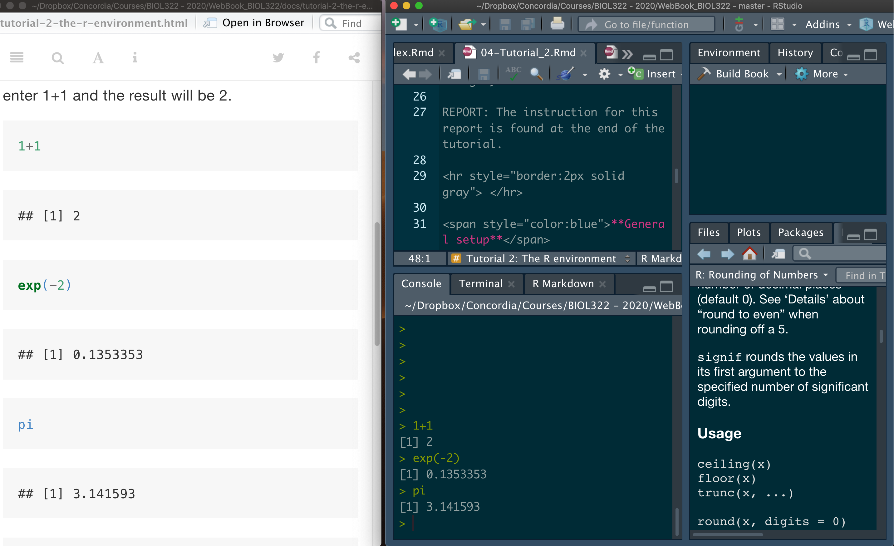
A good way to work through is to have the tutorial opened in our WebBook and RStudio opened beside each other.

Mean, median, variance, standard deviation & coefficient of variation

We will start the tutorial by using the data on Gliding snakes as seen in lecture 4.

Download the gliding snakes data file

First open the file “chap03e1GlidingSnakes.csv” in excel and try to understand how the data are organized.

Now upload and inspect the data. You probably noticed by now that the function View allows you to see all the data, including the names of variables (i.e., columns of the data matrix). The function head prints the first 6 rows of the data matrix and helps identifying the name of the variables in case you don’t remember them; knowing the names of variables is very important as you need to often refer to them during analyses. One often forgets variables names even when you created them.

Not that you could also use the function names to print only the name of the variables (i.e., column names of the data matrix).

snakeData <- read.csv("chap03e1GlidingSnakes.csv")
View(snakeData)
head(snakeData)
names(snakeData)

As you learned in tutorial 3, data matrices are usually organized by having variables as matrix columns. Here we have variable (column) snake indicating the number of each observational unit (i.e., individual snake); and variable undulationRateHz containing the speed (cycles per second for each snake). Again, there are several ways to assess variables in a matrix separately, but the easiest way here (as seen in tutorial 3) is probably to use the $ sign; in this case, the name of the data matrix precedes $ and the name of the variable of interest succeeds $.

Calculate location statistics:

mean(snakeData$undulationRateHz)
median(snakeData$undulationRateHz)

You can also save the values into a variable for later use:

mean.undulation <- mean(snakeData$undulationRateHz)
mean.undulation
median.undulation <- median(snakeData$undulationRateHz)
median.undulation

Calculate spread (often referred as dispersion) statistics - the function sd stands for standard deviation and the function var for variance.

sd(snakeData$undulationRateHz)
var(snakeData$undulationRateHz)

Coefficient of Variation - R does not have a default function that calculates the coefficient of variation, but we can do that easily as follows:

sd(snakeData$undulationRateHz)/mean(snakeData$undulationRateHz) * 100

We can also calculate the coefficient of variation (CV) as follows:

sd.undulation <- sd(snakeData$undulationRateHz)
sd.undulation/mean.undulation * 100

Obviously you can also save CV into a variable as follows:

CV.undulation <- sd.undulation/mean.undulation * 100

Let’s plot the frequency distribution of the data (i.e., histogram):

hist(snakeData$undulationRateHz)

Making the histogram looks better:

hist(snakeData$undulationRateHz, breaks = seq(0.8,2.2,by=0.2), col = "firebrick",xlab="Undulation rate (Hz)",main="")

You could have used argument main to insert a title for the graph that would appear at the top. Usually in reports and publications we use legends for graphs so that we left it empty, i.e., main=“” (i.e., nothing between quotes).

Note that the X and Y axes are not touching. By setting the arguments xaxs and yaxs for axes x and y, respectively, to “i” we can make them touch. i stands for “internal” as oppose to regular (which would be “r” for regular); we refer it as “internal” in the sense that you set the axes to a different configuration other than the standard. Get used, R has a great number of “idiosyncrasies”; or at least as many other languages (natural and computer languages). I often say: “don’t fight the language, accept it!”

hist(snakeData$undulationRateHz, breaks = seq(0.8,2.2,by=0.2), col = "firebrick",xlab="Undulation rate (Hz)",main="",xaxs = "i",yaxs="i")

Boxplots & interquartile range

Let’s use a different data set, the spider running speed data set (as seen in lecture 5).

Download the running spider data file

First open the file “chap03e2SpiderAmputation.csv” in excel and try to understand how the data are organized.

Upload and inspect the data:

spiderData <- read.csv("chap03e2SpiderAmputation.csv")
View(spiderData)
head(spiderData)
names(spiderData)

Note below that we changed the way we call variables. We will not use the $ sign. Some functions such as the boxplot also accept the name of the variables directly. In these functions, the name of the variables within the data matrix can be easily recognized as they use the argument data, facilitating typing and reducing the code:

boxplot(speed ~ treatment, data = spiderData)

Obsviously we could have used $ instead of simply using the argument data in the function above. It would seem a little bit of more work to type though:

boxplot(spiderData$speed ~ spiderData$treatment)

What is the problem with the boxplot? The issue is that the after speeds appear before the before speed. This is because these variables are not being treated as numerical but rather as strings (i.e., a sequence of characters) and as such the letter a comes before the letter b in the alphabet. In this case, we need to transform the variable treatment into a numerical code (referred as to factor in R) in which we can also change the order of their appearance. This is done by using the function factor. This function is quite useful and we’ll use it in several types of analyses and tutorials in BIOL322:

spiderData$treatment <- factor(spiderData$treatment, levels = c("before", "after"))

Now plot the histogram again; now before will appear before after; Ok, writing that was pretty circular but true!

boxplot(speed ~ treatment, data = spiderData)

Now, let’s make the boxplot look much nicer. It it easy to forget the arguments in most R functions, including the ones used in boxplot. So, here is some additional information that you will be able to use in the future to make boxplot nicer than the ones produced by the default function boxplot; argument boxwex controls the width of the boxes so that we can make them narrower; here boxwex was set to 0.5 but “play” with the value to see what happens.

The argument whisklty sets the type of line for the whiskers - setting it to 1 the whiskers appear as solid lines (and not as a dahsed line as in the default, i.e., in the way was generated in the earlier boxplot). Finally, argument las makes the labels of axes appear in different directions - try las=0, las=1 and las=2 to see what happens (try in class but no need to include in the report). Here we used las=1 (needed to be included in the report):

boxplot(speed ~ treatment, data = spiderData, ylim = c(0,max(spiderData$speed)),col = "goldenrod1", boxwex = 0.5, whisklty = 1, las = 1,xlab = "Amputation treatment", ylab = "Running speed (cm/s)")

Just by looking at the boxplot, you can notice that the distributions of before and after speeds are asymetric. Look into our lecture slides and try to figure out which type of asymmetric distribution each variable represents (right or left skewed). Write this information in the tutorial report code file (see below) as follows:

# before amputation the distribution type is "YOUR ANSWER" and after amputation the distribution type is "YOUR ANSWER".

Don’t forget to use the symbol # so that the text you wrote will not be interpreted as commands.

Because the data are quite asymmetric, we will use location and spread statistics based on median and quartiles, respectively, instead of mean and standard deviations. Here we have two groups in the data, i.e., before and after. In tutorial 3, we introduced the function aggregate. This function selects data belonging to a similar categorical value in a list (here treatment, i.e., before or after) and applies a function on the basis of these values separately. Here we will use the median per treatment, hence median as the third argument in the function aggregate. The median is then calculated for each group as:

aggregate(spiderData$speed, list(spiderData$treatment), median)

The use of the function aggregate with the function quantile is a bit “complex” (see below). To make it simpler, let’s create variables that contain the speed values before and after voluntary amputation separately. This is done using the function subset and setting its argument treatment as the name of the code used for each individual spider. Note that here, the argument treatment received a “==” instead of a “=”. Note that the double equal sign “==” is needed when using a logical statement indicating “is equal to” in R:

speedBefore <- subset(spiderData, treatment == "before") 
speedBefore
speedAfter <- subset(spiderData, treatment == "after") 
speedAfter

Now let’s calculate the median, 25% (Q1) and 75% (Q3) quartiles using a function called quantile in which we establish the values in the distribution in which quartiles are calculated using the argument prob. The word prob is used here (i.e., probability) because we are inferring that there is a 25% chance of finding a value equal or smaller than Q1 (which is based on the sample values) in the distribution of the entire statistical population of spiders (i.e., all male spiders of that species during mating season either before or after amputation)! and there is a chance equal to 75% chance of finding a value equal or greater than Q3. Note that here chance is based on the statistical populational concept in which the sample values are used to estimate population parameters. As such, we use the sample quartiles (Q1, Q2 & Q3) to infer about these two statistical populations: all male spiders of that species during mating season either before (population 1) or after amputation (population 2)

median(speedBefore$speed)
median(speedAfter$speed)
quantile(speedBefore$speed, probs = c(0.25, 0.75))
quantile(speedAfter$speed, probs = c(0.25, 0.75))

Note that the median Q2 of a distribution represents the value that divides the distribution of values into half; i.e., there is a 50% chance of finding a value equal or smaller than Q2; and a 50% chance of finding a value equal or greater than Q2 (i.e., prob for Q2 = 0.50); so that we could have calculated Q1, Q2 and Q3 just using the function quantile as follows:

quantile(speedBefore$speed, probs = c(0.25, 0.50, 0.75))
quantile(speedAfter$speed, probs = c(0.25, 0.50, 0.75))

The interquartile range (IQR) for both speeds (before or after) can be calculated using the function IQR as follows:

IQR(speedBefore$speed)
IQR(speedAfter$speed)

Remember that IQR = Q3 - Q1; so we could have equally calculated IQR as follows:

quantile(speedBefore$speed, probs = c(0.75))-quantile(speedBefore$speed, probs = c(0.25))
quantile(speedAfter$speed, probs = c(0.75))-quantile(speedAfter$speed, probs = c(0.25))

Learning and practicing R further using the stickleback lateral plates data

Let’s practice the concepts of location and spread statistics using yet a different data set. Often the nature of the data is different so that you can develop further an understanding of data structure and R by using different data. We will use the stickleback lateral plates data (lecture 6).

Download the stickleback data file

First open the file “chap03e3SticklebackPlates.csv” in excel and try to understand how the data are organized.

Upload and inspect the data:

sticklebackData <- read.csv("chap03e3SticklebackPlates.csv")
View(sticklebackData)
head(sticklebackData)

Next, calculate the mean for each genotype. As in real languages, theare are many ways to say something, including words that are synonyms. Instead of the function aggregate, here we will calculate IQR using the function tapply instead; we will also learn how to round values using the function round:

meanPlates <- tapply(sticklebackData$plates, INDEX = sticklebackData$genotype,FUN = mean)
meanPlates <- round(meanPlates, digits = 1)
meanPlates

Calculate the median for each group:

medianPlates <- tapply(sticklebackData$plates, INDEX = sticklebackData$genotype,FUN = median)
medianPlates <-round(medianPlates, digits = 1)
medianPlates

And the standard deviations for each group:

sdPlates <- tapply(sticklebackData$plates, INDEX = sticklebackData$genotype, FUN = sd)
sdPlates <- round(sdPlates, 1) 
sdPlates

The interquartile range by group:

iqrPlates <- tapply(sticklebackData$plates, INDEX = sticklebackData$genotype,FUN = IQR, type = 5)
iqrPlates

Let’s learn something new. Let’s produce a table containing the number of individuals for each genotype. Here we will use the function table as follows:

sticklebackFreq <- table(sticklebackData$genotype)
sticklebackFreq

The total number of individuals independent of the genotype can be calculated in several ways in R but here we can simply:

sum(sticklebackFreq)

The relative frequency of each genotype is given by:

sticklebackFreq/sum(sticklebackFreq)

Finally, let’s produce a boxplot; note how we simply changed the names of the variables we used in the 1st boxplot for the spider data - so pretty much a job of coyping and pasting and changing the variable names from your previous applications. This is often what we do in R, so keeping files organized and well explained makes it “half of the job done” in R!

boxplot(plates ~ genotype, data = sticklebackData, ylim = c(0,max(sticklebackData$plates)), col = "goldenrod1", boxwex = 0.5, whisklty = 1, las = 1, xlab = "Genotype", ylab = "Number of plates")

Miscellanea - Some advanced notes

If you are curious about developing stronger R skills, this will help you to practice it further. That said, you won’t need to use these functions in your reports.

Calculate Q1, Q2 and Q3 using the function aggregate for both speeds at the same time. The argument function (x) is used because the function quantile has probs as an argument.

aggregate(spiderData$speed, list(spiderData$treatment), function (x) quantile(x, probs = c(0.25, 0.50, 0.75)))

Note that the above is a little more complex . IQR could had been equally calculated for both speeds using aggregate in the usual way we learned how to use the function aggregate. Because we are not using arguments for the function IQR as we needed for the function quantile, we don’t need to use the argument function (x) in aggregate.

aggregate(spiderData$speed, list(spiderData$treatment),IQR)

We could also have calculated IQR using the function tapply (as seen earlier) as follows:

tapply(spiderData$speed, INDEX = spiderData$treatment, FUN = IQR)

and the more complicated usage of the function quantile as follows given that quantile requires the argument probs.

tapply(spiderData$speed, INDEX = spiderData$treatment, function(x) FUN = quantile(x, probs = c(0.25, 0.50, 0.75)))

Why all these different ways? As in natural languages, depending on the context, we may prefer to use different forms of expression depending on the circumstance, e.g., “I have a problem”, “I have an issue” or “I have a dilemma” all these may sound quite similar or different depending on the context! Functions in R as well. Here the functions tapply and aggregate were used to produce the same calculations as before, but each of then can do things that the other can’t depending on the circumstances.

ACADEMIC INTEGRITY & AVOIDING ACADEMIC MISCONDUCT. We hold the principles of academic integrity, that is, honesty, responsibility and fairness in all aspects of academic life, at their highest values.

Some of our tutorials take years to perfect and they are built to enhance your learning of Biostatistics. Some of the reports here are similar to previous years and you are not allowed to consult reports from students in this year or previous years. WE HAVE SOFTWARE that can calculate the similarity among reports from students this year and in past years. This may trigger academic infractions to you and those previous students that passed you their reports even after they graduate. Academic infractions can be brought on students even after they graduate and have their records modified to reflect past academic misconducts.

Using previous reports also demonstrates a complete lack of respect for the work of professors and instructors.

Report instructions

Describe a fictional biological problem (e.g., an experiment or observational study you designed) that has one quantitative variable. Observational units should be divided into two categories (e.g., male/female, genotype, freshwater/marine water, low/high pH, ar any type of categorical variable with two categories). Invent a data set (make up numbers) for the problem at hands and place them in a csv file. You can use excel and then save it in csv format.

Then create R code where the data files is read and you calculate mean, median, standard deviation, variance and the interquartile range for each category. Plot the boxplot as well. You can describe your fictional problem using # to comment the code; for example:

# I set up a study that .....
# use as many lines as necessary,
# always starting with  #
Code here:

Submit the RStudio file and the relevant csv file via Moodle. We have a lot of experience with tutorials and they are designed so that students can complete them at the end to the tutorial in question. No written report (e.g., in a word file) is necessary, just the two files.