Tutorial 5: Sampling variation

Sampling variation, uncertainty, sampling properties of the mean and standard deviation, the standard error of the mean and confidence intervals

Week of October 3, 2022
(5th week of classes)

How the tutorials work

The DEADLINE for your report is always at the end of the tutorial.

The INSTRUCTIONS for this report is found at the end of the tutorial.

Students may be able after a while to complete their reports without attending the synchronous lab/tutorial sessions. That said, we highly recommend that you attend the tutorials as your TA is not responsible for assisting you with lab reports outside of the lab synchronous sections.

Your TAs

Section 101 (Wednesday): 10:15-13:00 - John Williams (j.p.w@outlook.com)
Section 102 (Wednesday): 13:15-16:00 - Hammed Akande (hammed.akande@mail.mcgill.ca)
Section 103 (Friday): 10:15-13:00 - Michael Paulauskas (michael.paulauskas@mail.mcgill.ca)
Section 104 (Friday): 13:15-16:00 - Alexandra Engler (alexandra.engler@hotmail.fr)

General Information

Please read all the text; don’t skip anything. Tutorials are based on R exercises that are intended to make you practice running statistical analyses and interpret statistical analyses and results.

This tutorial will allow you to develop basic to intermediate skills in plotting in R. It was produced using code adapted from the book “The Analysis of Biological Data” (Chapter 2). Here, however, we provide additional details and features of many of the R graphic functions.

Note: At this point we are probably noticing that R is becoming easier to use. Try to remember to:

set the working directory
create a RStudio file
enter commands as you work through the tutorial
save the file (from time to time to avoid loosing it) and
run the commands in the file to make sure they work.
if you want to comment the code, make sure to start text with: # e.g., # this code is to calculate…

Intro video for tutorial 5 by Timothy Law (with input from the TA team). The video remains very useful even though it was produced in 2020. However, information about TAs and reports are no longer valid.

General setup for the tutorial
A good way to work through is to have the tutorial opened in our WebBook and RStudio opened beside each other.

Critical notes for this tutorial

Although you don’t need to memorize R commands, general information learned in tutorials may be asked in exams. For instance, explain the basis of the computational method used in this tutorial? See below!

This tutorial was planned to help you understand the nature and characteristics of sampling variation and sampling distributions. As we saw in our past lectures (7, 8 & 9), sampling distributions are key to understand and produce inference.

In this tutorial, you will learn only about the sampling distribution of the mean and the sampling distribution of the standard deviation. This is because they are the most important ones for statistical inference. Note that given that the standard deviation squared (\(s^2\)) equals the variance, the characteristics of sampling distributions of the standard deviation hold for the sampling distributions of the variance as well. That said, their shapes are different (we will see this later in the course).

TIP: We highly recommend that you take notes (preferably on paper) as you work through tutorials. This will allow you to better understand and take in what you are doing rather than just typing commands. I assure you that taking notes along the way will help you in the exams as well because you need to know the properties and characteristics of estimators (i.e., statistics based on samples such as the mean and standard deviation).

Computational versus analytical approaches to build sampling distributions

To understand what sampling distributions are and their properties, we will build sampling distributions computationally. In classic statistics, these distributions are built using calculus (i.e., analytically). What is important is that both computational and analytical methods give (for all purposes) the exact same results in terms of the concepts covered in this tutorial (and in general). The difference is that more than 100 years ago, when the statistical principles for inference based on sampling started being developed, computers did not exist and calculus was used. We still use analytical methods for most parts of Introduction courses in statistics. That said, computational methods are increasing in usage due to the complex nature of many biological problems.

The main reason we are using a computational approach here instead of an analytical one is that it will help you to understand more intuitively the concepts underlying sampling variation and sampling distribution. The analytical would requires greater knowledge of calculus and probability. Although we will learn these concepts computationally, we will apply them using analytical solutions that exist for decades (and some more than 100 years). Remember, they give you the same results (as we will demonstrate in later tutorials).

The tradition though is to apply statistics using the original methods (developed analytically). And analytical methods are still a bit faster since the theory is already built-in and doesn’t need to be developed (as we will do here) every time we want to apply a particular statistical method for inference.
Remember that the standard error is the variation around the sample statistics of interest (e.g., mean, standard deviation, etc). For now, we will focus on the standard error of the mean but one could calculate the standard error of any statistic of interest, including the standard error of the standard deviation, variance, median, etc.

Sampling variation based on a normal distribution

Either analytically or computationally, we need to assume a form for the population distribution so that samples can be taken (sampled) from it (often we also say “samples drawn from a population”).

Because the normal distribution is well characterized (i.e., its properties are well defined), we can generate (draw) samples from a normally distributed population using most statistical software including R (and even Excel). Most statistical software have “built in” random sampling generators for most common probability distributions (normal, uniform, log-normal, etc). However, the normal distribution is always the most commonly assumed as seen in our lectures. Interestingly, as we will see here and in other lectures, assuming that the values from the statistical population of interest are normally distributed, it does not mean that if the original population is not normal that the statistics we use will not work for inferential purposes.

Let’s start by understanding how to create a vector of random values drawn from a normal distribution. All the values generated and recorded in the vector are a single sample.

In statistics we say “to draw random values from a normal distribution” (or any other distribution of interest). Random sampling is assumed because each value is independent of one another (remember the principles of random sampling discussed in lecture 7). As I often say, there is one way to be independent (random sampling) but infinite ways in which samples could be dependent. As such, assuming random sampling makes analytical and computational solutions easier. That said, if sampling was not random, then statistical methods for inference can be biased (more on that later).

In the line of code below, the argument n sets the sample size, the argument mean sets the mean of the population of interest and the argument sd sets the standard deviation of the population (remember again that the standard deviation squared \(s^2\) is the variance of a distribution). A normal distribution is defined by its mean and its variance (or standard deviation). The normal distribution used here will be treated as the true population of interest! As such, the function rnorm allows us to sample from a normally distributed population with a given mean and standard deviation set by us. Let’s draw 100 values (i.e., a sample of 100 observations, i.e., n=100) from a normally distributed population with mean \(\mu\) = 20 and a standard deviation (\(\sigma\)) = 1.
Think of this normal distribution below as the distribution of trees in a forest where the true population mean (i.e., across all trees) is 20m and its standard deviation is 1. And below we will be sampling 100 trees randomly from that forest and measuring their heights. For all purposes though, the normal distribution has infinite number of observational units (i.e., infinite number of trees). Assuming statistical populations off infinite sizes is not an issue and works great for finite populations. For all purposes, analytically and computationally, statistical populations are considered infinite.

sample1.pop1 <- rnorm(n=100,mean=20,sd=1)
sample1.pop1

Let’s plot the frequency distribution (histogram) of our sample and calculate the sample statistics we will be working on today:

hist(sample1.pop1)
mean(sample1.pop1)
sd(sample1.pop1)
var(sample1.pop1) # or sd(sample1.pop1)^2

Let’s take another sample from the same population:

sample2.pop1 <- rnorm(n=100,mean=20,sd=1)
sample2.pop1
hist(sample2.pop1)
mean(sample2.pop1)
sd(sample2.pop1)
var(sample2.pop1) # or sd(sample2.pop1)^2

Notice how the values for the summary statistics (mean, standard deviation and variance) varied among samples? So, even though they were taken from the same population, samples vary in their values (data) and summary statistics. This is the principle of sampling variation we covered in lectures 7 and 8.

Let’s now generate a sample from another population with \(\mu\) = 20 and \(\sigma\) = 5 (a larger standard deviation than the value of \(\sigma\)=1 set for the previous population above):

sample1.pop2<-rnorm(n=100,mean=20,sd=5)
sample1.pop2

Let’s plot its frequency distribution (histogram) and calculate its mean and standard deviation:

hist(sample1.pop2)
mean(sample1.pop2)
sd(sample1.pop2)
var(sample1.pop2) # or sd(sample1.pop2)^2

Just to improve your knowledge of R, let’s plot where the mean value falls in the distribution using a vertical line; the argument lwd controls how thick the line is plotted.

abline(v=mean(sample1.pop2),col="firebrick",lwd=3)

Let’s compare the two samples by plotting their frequency distributions (histograms) of each sample on the same graph window using the function par. We will use this function to tell R that the plot will have two rows (one for each histogram) and 1 column, i.e., par(mfrow=c(2,1)). To plot 3 histograms on the same graph window we would set the function par as: par(mfrow=c(3,1)). To plot 4 histograms instead on the same graph window, two on the top row and two on the bottom row, we would set the function par as: par(mfrow=c(2,2)).

Here, we won’t make the histograms look nice as we just want to observe their differences. Note that to be able to observe the differences between the two samples, you need to make sure that the scales of axes x and y (set by the arguments xlim and ylim) are the same:

par(mfrow=c(2,1)) 
hist(sample1.pop1,xlim=c(0,40),ylim=c(0,50),main="Sample from Pop. 1")
abline(v=mean(sample1.pop1),col="firebrick",lwd=3)
hist(sample1.pop2,xlim=c(0,40),ylim=c(0,50),main="Sample from Pop. 2")
abline(v=mean(sample1.pop2),col="firebrick",lwd=3)

Note how both samples are more or less located at 20m (i.e., average of 20m) but that the trees in sample 2 vary much more among each other. We will go back to this issue later on today’s tutorial.

Once finished, set the graph parameters back to their default otherwise you will have problems generated new graphs:

dev.off()

From sampling variation to sampling distributions: the case of a population with a small standard deviation

Sampling variation is the variation in data and summary statistics from sample to sample from the same statistical population. Sampling distributions are the distribution of a particular statistic of interest (mean, variance, etc) across a really large number of samples. Analytically, this can be approximated via calculus. Computationally, we can do it as below.

A sampling distribution for any particular summary statistic of interest can be built by randomly drawing a large number of samples all with the same n (i.e., sample size) size from the same population (here normally distributed with a given mean and standard deviation; note again that other distributions certainly could be used). We keep the same n, because sampling distributions change as a function of sample size. And what we are trying to mimic is “and what if I had taken a different sample of the same size from the same population?”

It is very easy to draw multiple samples from any given population. We can use the function replicate to do that. Below we generate 3 random samples containing 100 observations (n=100) each from a normally distributed population with a population mean \(\mu\) = 20 and population standard deviation \(\sigma\) = 1:

happy.normal.samples <- replicate(3, rnorm(n=100,mean=20,sd=1))
happy.normal.samples

Note that the name of the matrix above can take any value. So why not happy.normal.samples?!

The dimension of the matrix is 100 observations (in rows) across 3 samples (each sample is in a different column):

dim(happy.normal.samples)

Let’s calculate the sample mean for each sample. For that, we will use the function apply. Each sample is in a different column; as such, we want then the MARGIN=2, i.e., calculate for each column. If we use MARGIN=1, then means are calculated per row of the matrix instead of the column. Finally, FUN here will be the mean.

apply(X=happy.normal.samples,MARGIN=2,FUN=mean)

Let’s go big now! Let’s take 100000 (one hundred samples). This should not take too long. I usually do one million or more but just to demonstrate the principles we are interested here, 100000 is fine.

lots.normal.samples.n100 <- replicate(100000, rnorm(n=100,mean=20,sd=1))

Calculate the mean for each sample and then plot the distribution of means.

sample.means.n100 <- apply(X=lots.normal.samples.n100,MARGIN=2,FUN=mean)
length(sample.means.n100)

See, there are 100000 sample means in the vector sample means. The frequency distribution contained in this vector of sample means (sample.means.n100) is called “the sample distribution of means”:

hist(sample.means.n100)
mean(sample.means.n100)
abline(v=mean(sample.means.n100),col="firebrick",lwd=3)

Note how small the variation is among sample means! Note also how the majority of them are closer to the true population mean of 20 m. This is because the distribution is symmetric. Finally, notice that the mean of these 100000 samples means is equal (for all purposes) to the population from which their samples were taken (i.e., \(\mu\) = 20)

The minimum and maximum values for the 100000 sample means are:

min(sample.means.n100)
max(sample.means.n100)

No sample has a mean that should be smaller than 19.2 or greater than 20.8. Wow!

Now, let’s get back to reality where only one sample is usually the case. Let’s say the first sample was the one that you sampled. And the others are just possible samples not sampled (see lecture 7 for details):

sample.means.n100[1]

Your value just above is probably a sample mean very very close to the true population. For instance, assume your sample mean was 19.84 m. So the error from the true population value would had been 0.16 m or only 16 cm (i.e., 20 m - 19.84 m) which is a tiny error given tall trees.

Can one trust this sample mean to make inferences then? That depends on the sampling distribution on unobserved sample means, i.e., all the other possible samples you could have taken from the population but you did not. But, if the majority of samples are closer to the true population mean, then your single sample will be likely too! That helps us to start building an understanding around the concept of uncertainty. Because most of the samples are closer to the true population value, then you could have a good level of certainty that your own sample mean is also close to the true population value. Note though, that so far we made the statement based on the fact that we know the true population value; which is almost never the case. But next we will understand that this statement may hold true also for samples from populations for which we don’t know their parameters; which are the majority of real cases in biology. But, by building theory around known populations help you understand generalizations to unknown populations.
In lecture 7 and 8, we discussed that the variation within a sample (standard deviation) can help estimating how confident one can be in how representative their sample is for the population. This is what we will learn in this tutorial.

Note that the population we considered above has a small mean relative to its standard deviation (CV = 1/20 = 0.05 = 5%); remember that we used a sample size of 100 trees.

Changing sample size. Let’s observe now what happens when sample size changes. Let’s say we sampled 30 trees instead of 100 trees. Should we be as confident in a single sample estimate based on 30 trees than in contrast to 100 trees?

Let’s estimate the sampling distribution for a sample size of 30 trees. Below we kept the same population (i.e., normal, mean=20 & sd=1). Population parameters were kept the same as before. All we have changed here is the sample size to 30 trees (instead of 100 trees):

lots.normal.samples.n30  <- replicate(100000, rnorm(n=30,mean=20,sd=1))
sample.means.n30 <- apply(X=lots.normal.samples.n30,MARGIN=2,FUN=mean)

Now let’s plot the two sampling distributions:

par(mfrow=c(2,1)) 
hist(sample.means.n100,xlim=c(18.5,21.5),main="n=100")
abline(v=mean(sample.means.n100),col="firebrick",lwd=3)
hist(sample.means.n30,xlim=c(18.5,21.5),main="n=30")
abline(v=mean(sample.means.n30),col="firebrick",lwd=3)

Note how the sample mean values are around the true population value (20 m). Let’s calculate that; i.e., let’s calculate the mean of sample means.

mean(sample.means.n100)
mean(sample.means.n30)

Note that they are for all purposes exactly the same as the population mean. We saw this property of sampling distributions of the mean in lecture 8.

But most importantly, note that from the sampling distribution (i.e., histogram of the frequency distribution of sample means), there is more variation among the sample means for samples based on 30 trees than 100 trees. Let’s calculate the standard deviation of sample means to measure this. Because the mean of sample means are the same for n=30 trees and n=100 trees, then we can compare these standard deviations directly.

sd(sample.means.n100)
sd(sample.means.n30)

What does these values tell us? For n=100, the standard deviation of sample means is more or less 0.099 m (~10 cm). That tells us that a sample mean value will differ by 10cm in average from the true population value; not bad if your trees are about 20m in average, right?

Which one is smaller? Obviously the standard deviation of sample means based on n = 100 trees. What is the standard deviation here? It is the average difference between the sample mean and the population mean. So, in average, sample means based on 100 trees are closer in average to the true population mean (20 m) than sample of 30 trees are. Obviously, there can be a few samples among the samples based on n=30 trees that are closer to the true population than a few of the samples based on n=100. But, in average, that’s not true as the standard deviation of the sampling distribution well demonstrates.
So, under random sampling, in average, we have greater certainty (i.e., it is more likely) that samples based on n=100 will be closer to the true population mean value than samples based on n=30. In other words, by chance alone based on random samples, there is greater chance (i.e., probability) that a single sample mean based on n=100 will be closer to the true population mean than one sample based on n=30 trees.

If you don’t clearly grasp yet what the standard deviation above is telling you, think this way: what is the probability that one single sample based on n=100 will be closer to the population mean than a single sample based on n=30 trees. First, let’s calculate the difference between the sample mean values and the population value:

diff.n100 <- sqrt((sample.means.n100-20.0)^2)
diff.n30 <- sqrt((sample.means.n30-20.0)^2)
dev.off()
boxplot(diff.n100,diff.n30,names=c("n=100","n=30"))

Note, again, that there is far more variation (as expected) when samples are based on n=30 than when based on n=100. How many samples are closer to the population value then?

length(which(diff.n100 <= diff.n30))/100000

So, there is about a probability of 68% that a single sample based on n=100 trees will closer to the true population value than based on a sample size of n=30.

Conclusion. Well, one has greater certainty (chance) of any given single sample being closer to the true population value for sample sizes that are relatively large (assuming observations, here trees, were randomly sampled from the population).

So, since we almost always have only one single sample, we can trust more our single sample based on 100 trees than 30 trees. Although we concluded this for a normally distributed population, this generalizes to other distributions type other than the normal distribution (e.g., uniform, lognormal, etc).

Accuracy & Precision
Let’s put what we have learned above into the perspective of accuracy and precision.

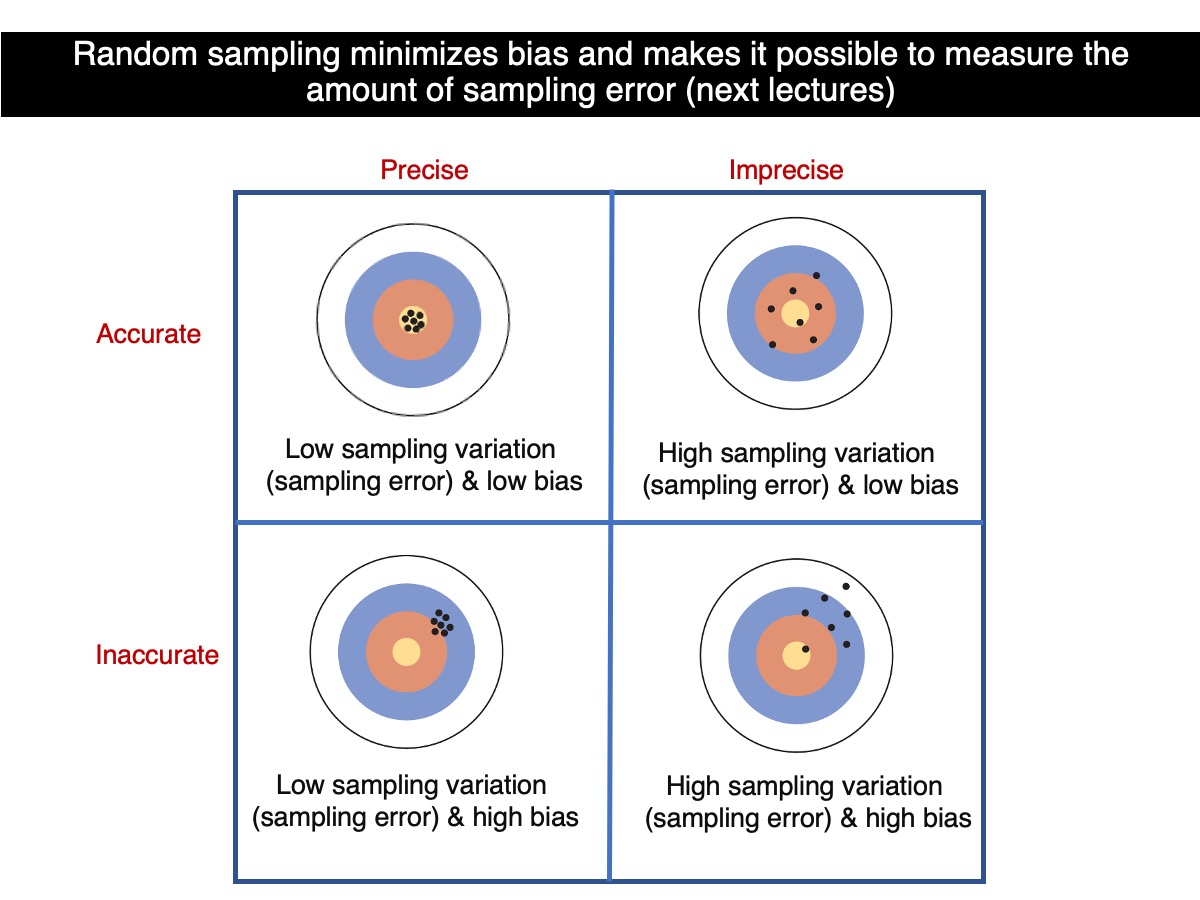
So, which sample size leads to greater accuracy? Samples based on 100 trees are in average more accurate than samples based on 30 trees. And which sample size size leads to greater precision? Also based on 100 trees because they are more similar in average to one another. So, as sample sizes increases, precision and accuracy do as well. All that assuming that random sampling was the case for all samples regardless of their sample sizes.

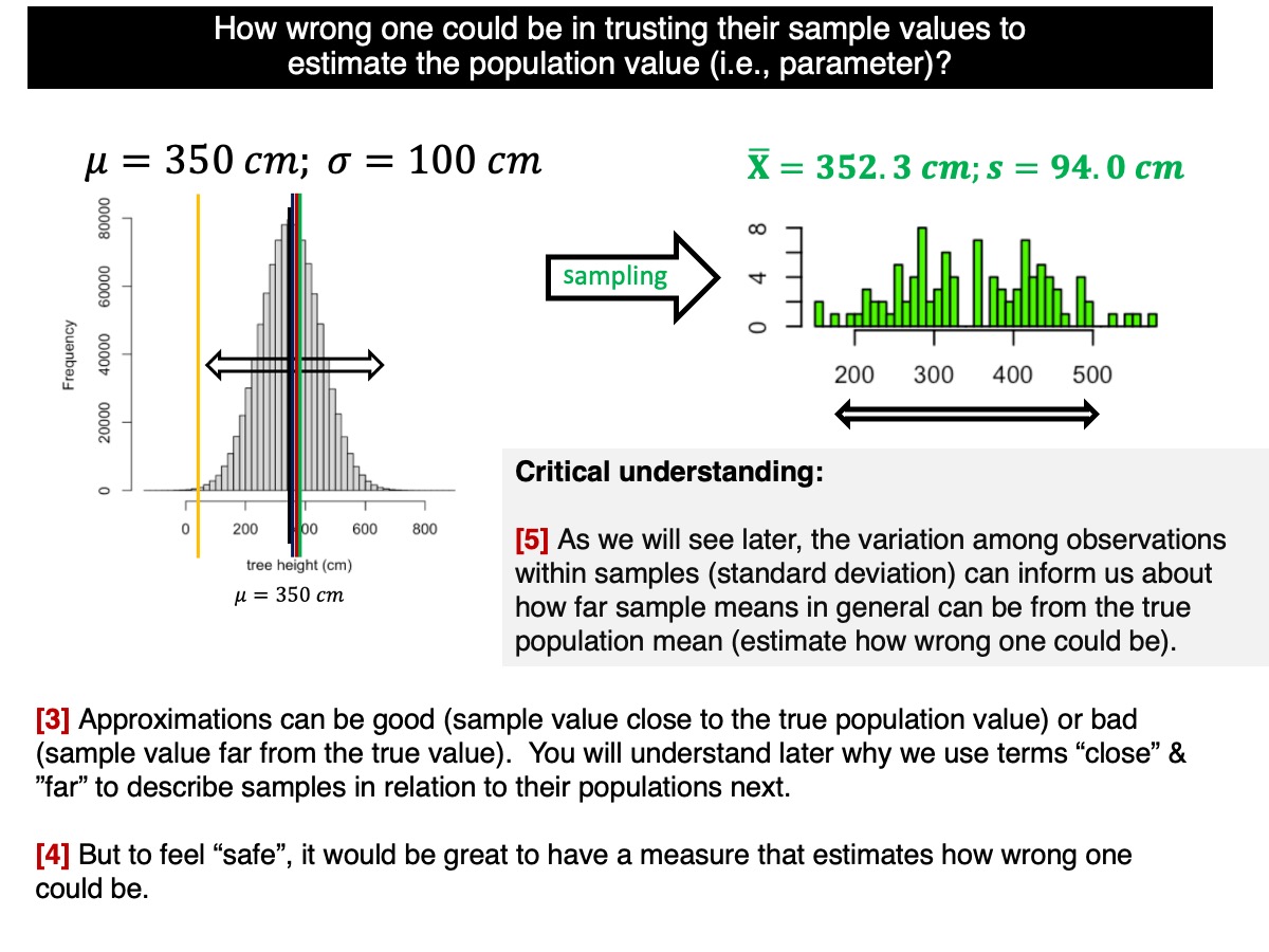
How to estimate uncertainty from one single sample?

As we mentioned and showed in our lectures, the variation among observations within samples (standard deviation of observations) can inform us about how far sample means can be from the true population mean (standard deviation of sample means, i.e., standard deviation for sample means from the population).

How does that work? Let’s go back to the standard deviation of the sample distributions (i.e., among sample means):

sd(sample.means.n100)
sd(sample.means.n30)

Remember that they are based on the variation of 100000 sample mean values around the true population value. And they are an estimate of the uncertainty (i.e., error) that we have around sample mean values. The standard error of the sampling distribution of means is called standard error (\(\sigma_\bar{Y}\)) and is one of the most important statistics and concepts in statistics. The standard error of the mean (\(\sigma_\bar{Y}\)) quantifies how accurately one can estimate the true mean of a population of interest. Now, if we divide the standard deviation of the population by the square root of the sample size, we get pretty much the same values as above:

1/sqrt(100) # = 0.1
1/sqrt(30)  # = 0.1825

They won’t be exactly the same (though pretty much the same) because we used 100000 samples; if we had used 1000000000 the differences would not be perceptible really. If we had then used infinite number of samples (given that the normal distribution as discussed earlier has infinite sizes), then the values would be exactly the same given the correspondent sample size.

All right, so what does that mean? We almost never know the true standard deviation of the population \(\sigma\) either. So how can we estimate how much sampling variation there is around the true population mean \(\mu\)? If the variation is high, then your should be less certain.

What we do though (and it works) is that one can estimate that error based on the standard deviation of a single sample. In other words, we can estimate the standard deviation of the sampling variation around the true population mean \(\mu\) based on the standard deviation of the sample. Wow! That’s statistics for you!

Let’s see how this works! Obviously there is also sampling variation around the true value of the standard deviation. So, let’s estimate standard errors from a single sample and understand how they can estimate how uncertain one can be; remember that lower uncertainty means high certainty (in average).

Let’s go back to the samples based on n=100 trees and n=30 trees. Remember that the mean of sample means equal the true population mean:

mean(sample.means.n100)
mean(sample.means.n30)

Let’s now estimate the standard deviation for each sample:

sample.sd.n100 <- apply(X=lots.normal.samples.n100,MARGIN=2,FUN=sd)
sample.sd.n30 <- apply(X=lots.normal.samples.n30,MARGIN=2,FUN=sd)

and plot their sampling distributions:

par(mfrow=c(2,1)) 
hist(sample.sd.n100,xlim=c(0,2),main="n=100")
abline(v=mean(sample.sd.n100),col="firebrick",lwd=3)
hist(sample.sd.n30,xlim=c(0,2),main="n=30")
abline(v=mean(sample.sd.n30),col="firebrick",lwd=3)

Boxplots could show their differences even better:

dev.off()
boxplot(sample.sd.n100,sample.sd.n30,names=c("n=100","n=30"))

Question - What did you notice? (no need to include the answer in the report)

First, the average of sample standard deviations is equal to the population standard deviation, i.e., 1 here.

mean(sample.sd.n100)
mean(sample.sd.n30)

The values above should be between 0.99 and 1.01; i.e., very close to the true population value. The reason (again) that the average of sample standard deviations does not equal exactly the population standard deviation is because we used 100000 samples and not a really huge (or infinite) number of samples. But you get the point!

Second, there is less sampling variation around the true population standard deviation for a large sample size as n=100 trees than n=30 trees.

So, the same patterns of variation related to sample size in terms of precision and accuracy for sample means apply to the sample standard deviation.

Let’s now go back to our original goal which was to have an estimate of uncertainty on a single sample. What we are doing here is to estimate error and based on that estimate, we assess how uncertain we are that our single sample will be a reasonable estimate for the true population mean value of tree heights. Statisticians opt for (as we will see during the course) words such as uncertainty and confidence; but not certainty. It may sounds semantics to you but it will become clearer during the course that it isn’t just simple semantics.

Remember that the standard deviation of the population divided by the square root of sample size measures the average error (uncertainty) of how the sample mean estimates vary around the true population mean. So, to estimate this error, we can then divide the sample standard error of the single sample we have by the square root of the sample size and use it as an estimate of the standard error.

Let’s observe that by dividing the sample standard deviations of the samples by their sample sizes, i.e., estimate for each sample what is the standard error of the sampling distribution of all sample means.

std.error.n100 <- sample.sd.n100/sqrt(100)
std.error.n30 <- sample.sd.n30/sqrt(30)

Let’s calculate their means:

mean(std.error.n100)
mean(std.error.n30)

No surprises there (well perhaps a bit). The average sample standard error equals the respective population standard errors, i.e., about 0.1 and 0.18.

Let’s put now all this “theory” into practice. Let’s pick the first sample in the series of samples of 100 trees:

sample.means.n100[1]
std.error.n100[1]

In my case, which will differ from yours, though the interpretation is the same among every one, the first sample mean based on n=100 trees was equal to 19.92 m and the standard error was equal to 0.103 m (10.3 cm). Remember that the standard error of the mean quantifies how precisely (from a precision point of view) you can estimate the true mean of the population. It tells you that, in average, the sample means will be about 0.103 m (or 10.3 cm) from the true population value. First, 0.103 m is pretty close to the true standard error of the population \(\sigma_\bar{Y}\); and tells us then that, in average, sample means differ from the true population mean \(\mu\) by 0.103 m (i.e., 10.3 cm).
Let’s put this into perspective. It follows then that if we add this estimate of the true average error \(\sigma_\bar{Y}\) (i.e., the sample standard error \(SE_\bar{Y}\) is assumed as a good approximation of the true standard error) around the sample mean value, we should have some expectation that the true population value for the mean \(\mu\) is within that interval. For my sample above, the value would be: 19.92 m - 0.103 m (19.817 m) & 19.92 m + 0.103 m (20.023 m), i.e., 19.92 m \(\pm\) 0.103 m. So, we have some expectation that the true value is in that interval.

The interval above is easy to calculate but not as easy to grasp (but not too difficult with some knowledge of symmetry of distributions; a conversation for another time). Let’s understand this computationally then. For how many sample means for which we could have sampled, the same interval will contain the true population value \(\mu\) = 20 m? Interestingly enough the one above did contain the true population values. Given that in reality we have no idea if we are right or wrong (we don’t know the true population value), we can really say in reality that my interval does contain the true population value. But, we can estimate estimate some certainty in which the confidence does contain the true population value.

Let’s start by building the interval for each sample mean. Remember the one for my sample (first in the vector out of 1000000), was 19.92 m \(\pm\) 0.103 m.

Left.value <- sample.means.n100 - std.error.n100
Right.value <- sample.means.n100 + std.error.n100

let’s plot the first 50 intervals:

n.intervals <- 50
plot(c(20, 20), c(1, n.intervals), col="black", typ="l",
ylab="Samples",xlab="Interval",xlim=c(19.5,20.5))
segments(Left.value[1:n.intervals], 1:n.intervals, Right.value[1:n.intervals], 1:n.intervals)

A good number of intervals contain (cross) the true population value, i.e., the horizontal bar crosses the vertical bar representing the true population mean value \(\mu\) = 20 cm. In other words that interval contains the true population mean value \(\mu\). But some intervals don’t contain \(\mu\). They are either to the left or to the right. How many in total out of 1000000 intervals contain the true population value? This can be calculated as:

length(which(cbind(Left.value <= 20.0 & Right.value >= 20.0)==TRUE))

In my case, there were 68254 out of 100000 that contained the true value of the population. This translates into a chance (probability) of 68.25% that the true population value is contained by one of the sample intervals simply built from sample values, i.e., sample mean \(\bar{Y}\) and sample standard deviation \(SE_\bar{Y}\).

CRITICAL: The above is not the same as to say that there is a probability of 68.25% that the calculated interval (based on a single sample) contains the true population mean. What is entailed is different. It entails that 68.25% of the calculated intervals (based on a single sample) will contain the true population mean (i.e., parameter). But any confidence interval either contains or it doesn’t contain the true population parameter. The probability doesn’t relate to a single interval but rather to the universe of intervals. That’s the reason why we say “confidence interval”; we should be confident that 68.25% of the intervals based on the sample will contain the true population value. Some intervals will be greater and some will be larger, but that doesn’t tell us whether one is more likely to contain the true population value. As we discussed in our lectures, confidence intervals are critical but often not well understood by practitioners.

We did not use any population value other than measuring how many of the sample-based intervals contained the true population value \(\mu\) = 20 m. Not bad. Let’s now consider an interval that’s is twice as big. So for my first sample that would had been 19.92 m \(\pm\) 2 x 0.103 m = 19.92 m \(\pm\) 0.206 m. So we are now assuming a marginal error of 0.206 around my original sample mean and it’s still quite small 20.6 m compared to my tree sample of 19.92 m. Let’s estimate the probability that such intervals contain the true population value:

Left.value <- sample.means.n100 - 2 * std.error.n100
Right.value <- sample.means.n100 + 2 * std.error.n100
length(which(cbind(Left.value <= 20.0 & Right.value >= 20.0)==TRUE))/100000

This probability is now much greater, in which about 95% of such (sampled based) intervals contain the true population mean and they were all estimated based on sample values. So, this is not too bad. If depending on the problem, we are fine with an error of 0.206 m, then we can say that we are highly confident (95% confident) that my sample interval 19.92 m \(\pm\) 0.206 m = 19.714 m and 20.126 m contains the true population mean! So, we can say that we are pretty confident that my sample mean value is a good estimate of the population value. However, as discussed above, we can’t say that any of the intervals has a probability of 95% of containing the true population value.

You will see in our lectures and the next tutorial, that the value we multiply by the standard error to estimate confidence intervals is not exactly 2; it will be a value that will change with sample size and we will see this later in our lectures and future tutorials. But multiplying by 2 (“a rule of thumb”), it gave you a good idea what is behind a confidence interval and how to estimate uncertainty with some certainty.

This is a long tutorial involving critical concepts that you need to understand to really understand what we do in statistics. Our course is built for you to understand these concepts as we move along.

Report instructions

The report is based on the following problem:

Create code in which you compare the sampling distribution of means for a normally distributed population with a mean of 25 m and a standard deviation of 2 m against a population with also a mean of 25 m but a standard deviation of 6 m.

Now answer: Which population has the greatest chance of having a sample mean the closest from the true population mean (i.e., parameter mean)? Demonstrate your answer using the code you developed above. Consider sampling distributions only; no need to consider confidence intervals.

Write text explaining your answer on the basis of the code and the concepts you have learned above.

# remember text (not code) always starting with  #

Submit the RStudio file via Moodle. We have a lot of experience with tutorials and they are designed so that students can complete them at the end to the tutorial in question.