Tutorial 2: The R and RStudio environments
Week of September 12, 2022 (2nd week of classes)
How the tutorials work
The in-person lab sections start this week. The one last week (tutorial 1) was asynchronous. This week’s tutorial is number 2. Tutorials = Labs; we use these terms interchangeably. Lab/Tutorial attendance is not mandatory but reports are.
The DEADLINE for your report is always at the end of the tutorial.
The INSTRUCTIONS for this report is found at the end of the tutorial.
Students may be able after a while to complete their reports without attending the in-person lab/tutorial sessions. That said, we highly recommend that you attend the tutorials as your TA is not necessarily responsible for assisting you with lab reports outside of the in-person lab sections.
Your TAs
Section 101 (Wednesday): 10:15-13:00 - John Williams (j.p.w@outlook.com)
Section 102 (Wednesday): 13:15-16:00 - Hammed Akande (hammed.akande@mail.mcgill.ca)
Section 103 (Friday): 10:15-13:00 - Michael Paulauskas (michael.paulauskas@mail.mcgill.ca)
Section 104 (Friday): 13:15-16:00 - Alexandra Engler (alexandra.engler@hotmail.fr)
General Information
This tutorial is meant to help you get acquainted with the R environment for statistical computing and its basic commands, ways to handle data and plot graphs.
Intro video for tutorial 2
by Timothy Law (with input from the TA team)
General setup for the tutorial
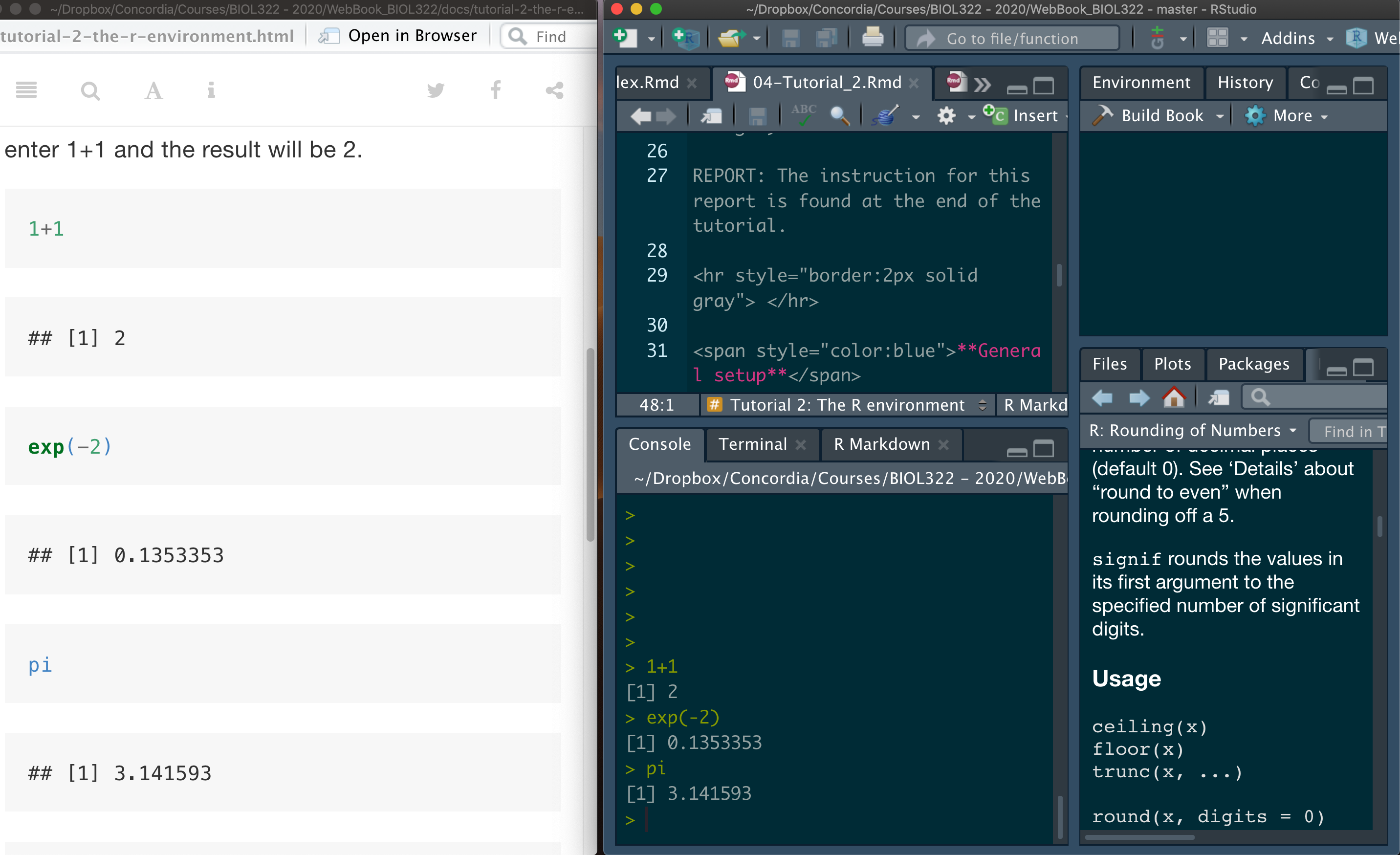
A good way to work through is to have the tutorial opened in our WebBook and RStudio opened beside each other. Note that the results from codes appear after ## (two hashtags) only in our tutorials and not in RStudio. We will not always present the results from operations in tutorials. This is often useful for demonstration purposes only.
Your first R steps
This tutorial was produced using some code adapted from “R and Data Mining: Examples and Case Studies” by Yanchang Zhao (2013); and also from Raphael Gottardo from his lectures in R and basic statistics (Exploratory Data Analysis and Essential Statistics using R).
Below you will find results of operations. Results below are shown with a ## in the beggining of the output. In the first set of commands below, you will enter 1+1 and the result will be 2. Results are shown with ## beside them.
1+1## [1] 2exp(-2)## [1] 0.1353353pi## [1] 3.141593exp(10)## [1] 22026.47round(3.123,digits=0)## [1] 3round(3.123,digits=2)## [1] 3.12round(sin(178.54),digits=3) # you can use functions together, i.e., pi, sin and round to produce a final value ## [1] 0.506sqrt(10)## [1] 3.162278Obs: the symbol # is used to annotate the code (make comments) so that whatever text appear after # is not interpreted by R when you hit
Assigning values to a variable (note that variable in computer programming is not the same as a variable in statistics as seen in class). In computer programming (Wikipedia) “Variable or scalar is a storage location (identified by a memory address) paired with an associated symbolic name (an identifier), which contains some known or unknown quantity of information referred to as a value.”
x=2 # variable here is x and it contains the number 2
y=2
x+y
## [1] 4c=2Creating a sequence of numbers:
x=0:5
x
## [1] 0 1 2 3 4 5Note that a large number of R users do not use the symbol = but rather <- which is the “assign” operator; this will not appear immediately useful to you in this course, but be aware when reading R material online and in this course, we tend to use <- instead of = but either is fine for all purposes of this course and programming in R.
Re-creating a sequence of numbers now using <-:
x<-0:5
x
## [1] 0 1 2 3 4 5It’s the same thing!
Your first plot in R:
x<-1:7
x
## [1] 1 2 3 4 5 6 7y<-11:17
y## [1] 11 12 13 14 15 16 17plot(x,y)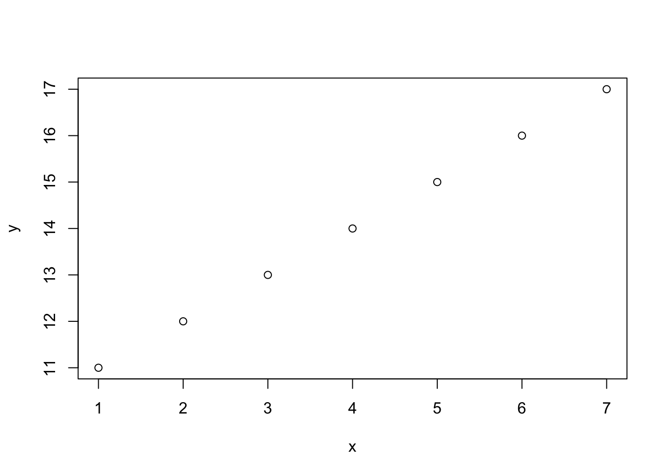
Let’s plot the same graph but with red dots instead of black as above:
plot(x,y,col="red")
Note that the vectors x and y did not need to be redifined because they are saved in the computer memory. Once you close R, these vectors are erased from the memory. You will learn later how to save scripts so that you don’t have to retype commands (see below). We can also save the values in the memory (later tutorial).
Creating a series of numbers (in a vector) by using function c (for combine values):
x <-  c(2,3,5,2,7,1)
x
## [1] 2 3 5 2 7 1More on calculations and dealing with vectors;
weight <- c(60,72,75,90,95,72)
# calling a particular cell
weight[1]
## [1] 60weight[2]## [1] 72weight## [1] 60 72 75 90 95 72height <- c(1.75,1.80,1.65,1.90,1.74,1.91)
bmi <- weight/height
bmi## [1] 34.28571 40.00000 45.45455 47.36842 54.59770 37.69634Les’t calculate the mean of a series:
(1+2+3+4+5)/5## [1] 3The power of R is that scripted functions are used to calculate metrics of interest and conduct statistical analyses. Two examples:
sum(height)## [1] 10.75mean(height)## [1] 1.791667We will learn lots of functions in BIOL322.
R allows to allocate values calculated by functions (such as the mean) to a variable; note that you can give any name to a variable. Here I used mean.x to make it more intuitive; but you could have used doNotGetDistracted (or whatever really) instead:
mean.x<-mean(height)
mean.x
## [1] 1.791667doNotGetDistracted<-mean(height)
doNotGetDistracted## [1] 1.791667We can sort values in ascending order:
sort(x) ## [1] 1 2 2 3 5 7or descending order:
sort(x,decreasing = TRUE) ## [1] 7 5 3 2 2 1Above, we learned something about R functions; they have “default” modes; the default mode of the function sort is to rank numbers in ascending order. BUT, you can change the default mode by switching the parameter “decreasing” to TRUE. As such, the default of the parameter “decreasing” in the function sort is FALSE. This can be found by asking information about the function as follows:
? sortWe will learn a lot about functions in the tutorials, so don’t worry for now about their defaults and how they work; this will be covered step-by-step as we learn more about R during our tutorials.
Reading data files
Let’s learn now how to read a file containing data. Download the file example_file.csv:
this file is in the widely used csv format that can be produced by excel among other programs; CSV stands for comma-separated values (CSV). This format is widely used: https://en.wikipedia.org/wiki/Comma-separated_values. R can read several types of file formats, but csv and text (.txt) are likely the most commonly used formats and csv is the preferred format in BIOL322.
Open the file in excel to take a look into how it is structured. Two variables
The function read.csv reads a file having an CSV format and saves the data into a variable (below we called this variable my.first.data). The option file.choose() tells R to open a window in which you can simply click and choose the file. But there are other ways to read files. This is the simplest when you are beginning to learn R.
my.first.data<-read.csv(file.choose())
my.first.data
Let’s open the data in a window in which you can see the values in a much better format
View(my.first.data)Often data is quite large (lot’s of rows) and you want just to observe the first few rows and see the names of variables (columns):
head(my.first.data)Let’s produce a scatter plot of the data:
plot(wingSize~bodySize,data=my.first.data)
A small tour in RStudio
The standard interface for R is often considered a bit raw and RStudio offers a more friendly interface to facilitate working with R.
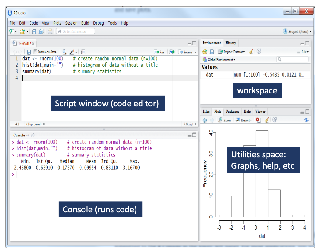
The four corners of RStudio
RStudio has four general windows to better distribute the different types of operations we can perform with R (code production, running code, graph output, data manipulation, etc).
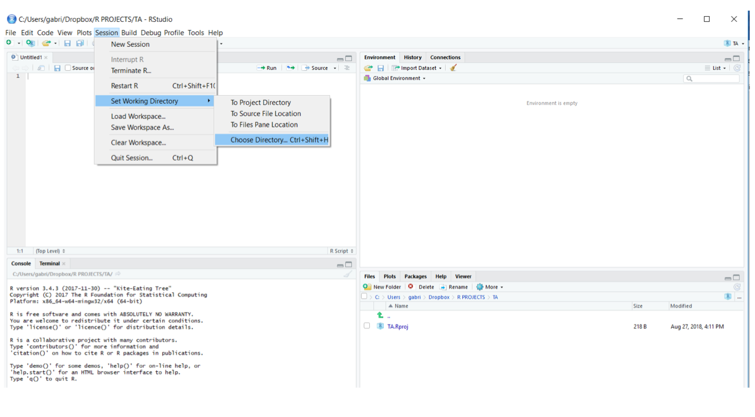
How to set the working directory
The “Working Directory” is the folder where R will search, by default, for files you want to open (e.g., data files, scripts) and where files that you create will be saved. In RStudio you can set your Working Directory either going to “Session -> Set Working Directory -> Choose Directory…”. Often is best to create different directories for different projects.
How to create and save R scripts
Entering and running code at the R command line is quite intuitive. However, this practice has its drawbacks given that you must re-enter your set of commands every time that you want to execute them. This issue is easily solved by creating and saving R scripts.
This is the way we will work in BIOL322. R scripts are files containing sets of commands and comments. These scripts can be saved and for later use such as re-running commands from previous analyses; or copying them so that you can adapt previous R scripts to new data or applications. Think about R scripts as a blank canvas where you can structure your analyses, make notes about your code and decisions you made during coding. This will become clearer as you gain more experience with R.
To create a new empty script in RStudio, click on the “New File” icon in the upper left of the RStudio main toolbar and select R script (see figure below). Once the new script is created, it is ready for code entry in the console tab.

How to execute R scripts
To execute the code written (i.e., Input) in an R Script, you must select the line and use the shortcut CTRL+ENTER in Windows or cmd+enter in MacOS. You will see the outputs of your code in the console tab. See a screenshot below.

Notice how RStudio places a number in front of each line of the code. As you will understand later, these numbers become helpful to visualize multiple outputs, particularly when using more complex codes.
Saving your recently created R script is quite simple. You can do it by clicking on the Save icon at the top of the script editor panel or through the shortcut CTRL+ S (or cmd+S). Opening a previous R session is also easy. You can either click on “File -> Open File” or use the shortcut key CTRL+O.
Importing data into R
In common applications, we use a data format called csv (comma separated ). Data in excel, for instance, can be saved in csv. To import data into RStudio is fairly simple using the function read.csv().In this example, we will assign our dataset (here, the file example_file.csv) to an object “mydata” using <- (an arrow formed out of < and - ).
mydata <- read.csv(“example_file.csv”)
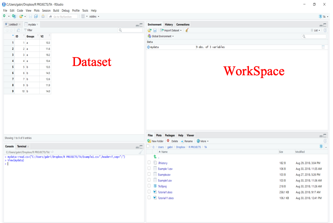
Once the object mydata is created, it will automatically appear in your Working Space (upper right window in RStudio). To view your dataset, you can click on the object or use the function View() in the console as follows:
View(mydata)
Exporting files from R
During the tutorials and course work, you will need to export data or results generated in R and save them in different formats csv format. The function write.csv() allows you to create files that will be automatically saved in your Working Directory. Example:
write.csv(my.first.data, file= "body.csv", row.names = FALSE)Stating the argument row.names as FALSE, it avoids generating an extra columns with row numbers in the saved file. This may be useful in other applications.
Saving and loading workspaces
You can save the objects (variables, matrices, results of analyses, etc) currently loaded into RStudio using the function save.image(). The combinations of objects during an R session is called “workload”. By typing in the console save.image(file=“Tutorial.RData”), you will save the workload. Using the command load(“Tutorial.RData”), you can reload all your previously work contained in that workspace.
You will learn lots more about R and graphs in the tutorials. For now, you have finished your first tutorial! Don’t hesitate to ask additional questions to your TA.
Report instructions
Reports are based on solving a few tasks using R. Everything you need to solve these tasks is based on simple adaptations of the codes you learned in that particular tutorial. Write all the code in an RStudio file, save it and submit it via Moodle. Submit also the csv file created below. Again, it is not mandatory that you attend the tutorials in person, but you are always required to complete their respective reports according to their deadlines. No written report (e.g., in a word file) is necessary.
The report should consist of the following
Create 2 series of 8 numbers each (any numbers you want) using the
ccommand as learned above.Calculate the mean (using the function mean seen above) of each series.
Plot them using the command plot above.
Create a csv file with 7 rows and two columns representing two variables, nitrogen and temperature. Plot these values where temperature is in the Y axis and nitrogen in the X axis.
That’s your report for today!