Tutorial 6: Sample estimators

Biases and corrections in the estimation of sample standard deviations, and confidence intervals in practice

Week of October 17, 2022
(6th week of classes)

How the tutorials work

The DEADLINE for your report is always at the end of the tutorial.

The INSTRUCTIONS for this report is found at the end of the tutorial.

Students may be able after a while to complete their reports without attending the synchronous lab/tutorial sessions. That said, we highly recommend that you attend the tutorials as your TA is not responsible for assisting you with lab reports outside of the lab synchronous sections.

The REPORT INSTRUCTIONS (what you need to do to get the marks for this report) is found at the end of this tutorial.

Your TAs

Section 101 (Wednesday): 10:15-13:00 - John Williams (j.p.w@outlook.com)
Section 102 (Wednesday): 13:15-16:00 - Hammed Akande (hammed.akande@mail.mcgill.ca)
Section 103 (Friday): 10:15-13:00 - Michael Paulauskas (michael.paulauskas@mail.mcgill.ca)
Section 104 (Friday): 13:15-16:00 - Alexandra Engler (alexandra.engler@hotmail.fr)

General Information

Please read all the text; don’t skip anything. Tutorials are based on R exercises that are intended to make you practice running statistical analyses and interpret statistical analyses and results.

This tutorial will allow you to develop basic to intermediate skills in plotting in R. It was produced using code adapted from the book “The Analysis of Biological Data” (Chapter 2). Here, however, we provide additional details and features of many of the R graphic functions.

Note: At this point we are probably noticing that R is becoming easier to use. Try to remember to:

set the working directory
create a RStudio file
enter commands as you work through the tutorial
save the file (from time to time to avoid loosing it) and
run the commands in the file to make sure they work.
if you want to comment the code, make sure to start text with: # e.g., # this code is to calculate…

General setup for the tutorial
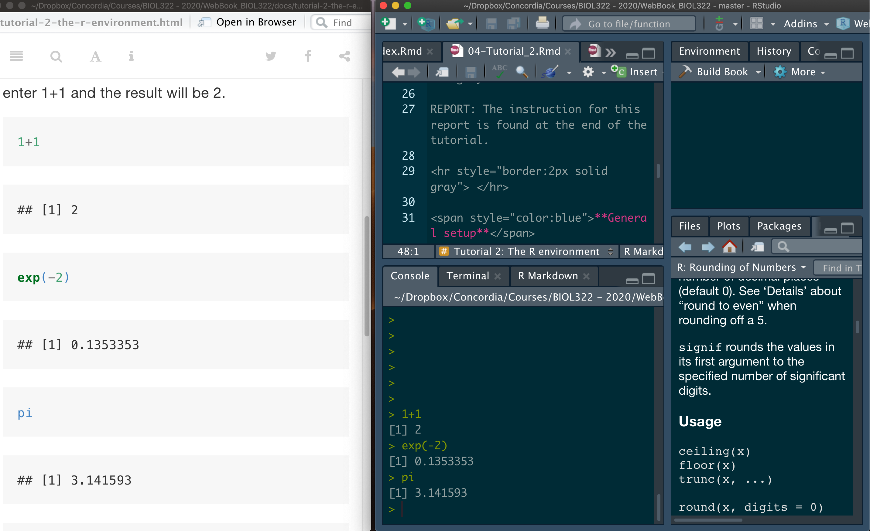
A good way to work through is to have the tutorial opened in our WebBook and RStudio opened beside each other.

This tutorial is based on lecture 11, which, for some lab sections, it takes place afterwards (i.e., this coming Thursday). This poses no issues as the the lecture and tutorial are quite interrelated and the issues covered in lecture 11 are extensively covered in this tutorial as well

Demonstrating the importance of sample corrections and degrees of freedom

One of the concepts that is often difficult to understand is the concept of degrees of freedom and the need of corrections to make sample estimates accurate and not biased. Remember that for the purposes of this course and standard basic and advances applications of statistics, an accurate sample estimator is one that the average of sample values for the statistic of interest equals the population parameter of interest. This applies to any estimator. We have already covered that the average of all sample means equal the population mean. Let’s look into another statistic, the standard deviation so that you have a good understanding of what non-biased (or accurate estimators are). And if they are not, statistical researchers then need to create ways (often called corrections) to remove the bias in the sample estimator.

Let’s start by remembering what the formula for the standard deviation is:

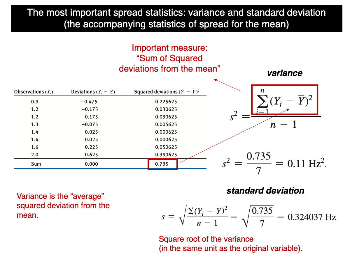
In words, it is the squared root of the sum of the squared differences (SS) between each value in the sample and the sample mean squared, divided by n-1. Most students that see this for the first time finds it odd and often question why SS is not divided by n instead of n-1. The n-1 is a correction necessary to make the sample variance an accurate (non-biased) sample estimate of the true population variance. This is known as the Bessel’s correction (https://en.wikipedia.org/wiki/Bessel%27s_correction). Let’s use a computational approach to demonstrate the fact that the variance based on n is a biased estimator but when based on n-1, it becomes unbiased.

The function ‘var’ in R is already based on n-1. This function could be equally entered “by hand” as follows. Note that the function rnorm considers the standard deviation of the population. So, if we set sd=2, then the variance of the population equals 4.

quick.sample.data <- rnorm(n=100,mean=20,sd=2)
var(quick.sample.data)
var.byHand <- function(x) {sum((x-mean(x))^2/(length(x)-1))}
var.byHand(quick.sample.data)

Note that our function by hand and the standard R function var gives exactly the same results. Notice also that, as such, we can use R to program our own functions (i.e., use R as a programming language).

Now let’s make a function in which the standard deviation is calculated using n in the denominator instead of n-1:

var.n <- function(x){sum((x-mean(x))^2)/(length(x))}
var.n(quick.sample.data)

Note that value calculated based on n is obviously smaller than the value based on n-1. Let’s see this in the context of sampling estimation bias.

Let’s draw 100000 samples from a normally distributed population with a sample size of n=20, population mean equal to 31 and variance equal to 2, i.e., standard deviation set as 4 for the population.

lots.normal.samples.n20 <- replicate(100000, rnorm(n=20,mean=31,sd=2))

For each sample, calculate the variance based on n-1 and n:

sample.var.regular <- apply(X=lots.normal.samples.n20,MARGIN=2,FUN=var)
sample.var.n.instead <- apply(X=lots.normal.samples.n20,MARGIN=2,FUN=var.n)

Let’s calculate the mean of all sample variances based on n-1 and n.

mean(sample.var.regular)
mean(sample.var.n.instead)

Note that the mean based on n-1 is extremely close to 4, i.e., the population parameter (not perfectly because we took 100000 samples instead of infinite). But the mean based on n is much smaller, demonstrating that the correction is necessary due to the issue of degrees of freedom that are covered in lecture 11.

That said, although the variance based on n-1 is not biased, the standard deviation based on n-1 is biased because the expected value (mean of all possible sample standard deviations) is not equal the true population standard deviation. Let’s see this issue in practice:

sample.sd.regular <- apply(X=lots.normal.samples.n20,MARGIN=2,FUN=sd)
mean(sample.sd.regular)

The population standard deviation is 2 and the value above is a bit smaller (~1.97) and, as such, it is biased. This bias has to do with the square root transformation of the variance and due to its mathematical complexity, we won’t cover it in too many details. It is difficult to establish a general unbiased procedure for the standard deviation as it will change as a function of sample sizes. However, there are attempts to do so (not covered in our course and it is a much more advanced procedure). Although there are corrections for this bias for normally distributed population, the bias “has little relevance to applications of statistics since its need is avoided by standard inferential procedures” that will be covered lates in the course:
https://en.wikipedia.org/wiki/Unbiased_estimation_of_standard_deviation

So, even though the sample standard deviation is a bit biased, we can trust that the sample standard deviation will serve useful in most applications of statistics (not all, but these applications are really advanced). In lecture 10, we saw that the t-distribution, which is used for calculating confidence intervals, was built using the sample standard deviations of samples. So, the bias of sample standard deviations is already integrated in the t-distribution. Note also that the bias depends on the sample size. When sample sizes are large, there is very little bias in sample standard deviations (i.e., as the t-distribution becomes narrower).

Just for curiosity, if the population is normally distributed, the sample standard deviation can be corrected by dividing it by a constant that is based on a complex statistical theory. The correction (as mentioned above) is not applied in general (no need) and the general theory that allows one calculating this constant won’t be covered in BIOL322. But I feel that showing it to you, it can increase your knowledge about what statistics involve:

mean(sample.sd.regular/0.986)

Note that the correction for n=20 is around 0.986. Once each standard deviation is divided by this constant, the standard deviation is now an accurate (unbiased) estimator of the true population standard deviation. Note how the mean of corrected standard deviations (above) is now is pretty much 2. If infinite samples were taken, than it would have been exactly 2.

The value of a sample estimator depends on the distribution of the population

Unlike the sample mean, which is not biased regardless of the shape of the population distribution (e.g., normal, uniform, asymmetric, bimodal, etc), it’s not possible to find an estimate of the variance that is truly unbiased for all types of distributions. The Bessel’s correction works well for normally distributed population or very close to normal. Let’s use the Human Gene Length data (20290 genes) to demonstrate the issues just described. Remember (as seen in our lectures) that we can assume the gene data to be the population data.

Download the gene data file

Now load the data in R as follows:

humanGeneLengths <- as.matrix(read.csv("chap04e1HumanGeneLengths.csv"))
View(humanGeneLengths)
dim(humanGeneLengths)

The mean and variance of the population are:

mean(humanGeneLengths)
var(humanGeneLengths)

Look at the distribution of the data and notice how asymmetric the distribution is:

hist(humanGeneLengths,xlim=c(0,20000),breaks=40,col='firebrick')

We will use the gene data to demonstrate the importance of the distribution of populations when using sample estimators. In this case we have the entire population, but the principle we will learn here applies to any unknown population which is what we usually have.

Let’s learn first how to take a sample from this population. For that we can use the function sample. The argument used here is size (here set to a sample size of n=100 genes):

geneSample100 <- sample(humanGeneLengths, size = 100)
geneSample100

Now let’s assess the statistical properties of sample estimators (mean and variance here) by taking multiple samples (100000) of sample size n=100 from the gene population; and then assess whether the sample mean and the sample variance are unbiased estimators.

geneSample100 <- replicate(100000, sample(humanGeneLengths, size = 100))
dim(geneSample100)

Let’s calculate the mean and variance for each sample:

gene.sample.means <- apply(geneSample100,MARGIN=2,FUN=mean)
gene.sample.var <- apply(geneSample100,MARGIN=2,FUN=var)

And let’s compare the mean of all sample values with the population parameters:

c(mean(gene.sample.means),mean(humanGeneLengths))
c(mean(gene.sample.var),var(humanGeneLengths))

Note that the difference between the mean of sample means and the population mean (i.e., all genes) is tiny but not the difference for the variance. And we know, the accuracy of the sample mean does not depend on the distributional properties of the population. In my samples, the difference between the mean of all sample means and the mean of the population was 2621.334-2622.055 which is tiny (-0.721; 0.721 / 2622.055 = 0.00027). Again, this is due to the fact that we did not take all possible samples and used instead 100000. Now, for the variance, the difference between the mean of all sample variances and the population variance in my 100000 samples was 4129115-4149425 (=20310) which is large than what we observed for the mean (i.e., 20310 / 4149425 = 0.004894). If we divide the two errors according to their proportions, we get 0.004894/0.00027 = 18.12593 times more error for the variance than the mean; i.e., the variance error is about 18 times than the error for the mean. Therefore the sample variance is a biased (not accurate) estimator for this asymmetric population. Note, though, that the variance is an unbiased estimator for normally distributed population as we saw above in the first part of this tutorial.

As such, we can’t trust the sample variance as an estimator for the population variance for populations that are not close to normally distributed.

Transformations can often remove the bias in sample estimates

Data transformation is well used to deal with statistical biases, including those biases generated by the fact that the distribution of statistical populations from where we sampled are not normal. Let’s apply the log-transformation here to see how it improves estimating the population variance for the gene population.

Let’s start by observing how the log-transformation affect the distribution of the population:

log.Genes <- log(humanGeneLengths)
hist(log.Genes,breaks=40,col='firebrick')

Note how the distribution is much more symmetric now. The mean and variance of the population log-transformed are:

mean(log.Genes)
var(log.Genes)

Let’s repeat the same process as before but we now log-transform the sample.

geneSample100 <- replicate(100000, sample(humanGeneLengths, size = 100))
gene.sample.means.log <- apply(log(geneSample100),MARGIN=2,FUN=mean)
gene.sample.var.log <- apply(log(geneSample100),MARGIN=2,FUN=var)

And let’s compare the mean of all sample values with the population parameters log-transformed:

c(mean(gene.sample.means.log),mean(log(humanGeneLengths)))
c(mean(gene.sample.var.log),var(log(humanGeneLengths)))

Notice how similar they are now after the log transformation. Using estimates based on transformations such as log and square-root (and many others) are widely used to improve accuracy of sample estimators.

Using the t-distribution to calculate confidence intervals

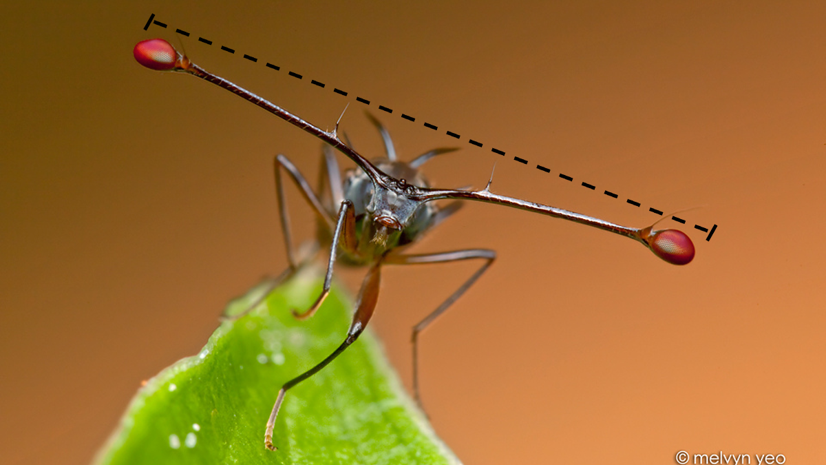
Let’s use a data set containing the span of the eyes (in millimeters) of nine male individuals of the stalk-eyed fly.

Download the stalk-eyed fly data file

Upload and inspect the data:

stalkie <- read.csv("chap11e2Stalkies.csv")
View(stalkie)

Let’s plot the histogram for the data. As you will see, the data look relatively symmetric. For now, this gives us a good indication that the distribution of the data is normally distributed so that we can use its sample standard deviation as am estimate of the true population standard deviation. As we saw in lecture 10, confidence intervals are calculated on the basis of the t-distribution.

We’ll see later in the course how to assess the assumption of normality in a more rigorous way.

hist(stalkie$eyespan, col = "firebrick", las = 1, 
    xlab = "Eye span (mm)", ylab = "Frequency", main = "")

Mean and standard deviation for the data:

mean(stalkie$eyespan)
sd(stalkie$eyespan)

Using the t-distribution, the 95% confidence interval for the population mean is:

t.test(stalkie$eyespan, conf.level = 0.95)$conf.int

The lower and upper limits of the interval appear in the first row of the output, i.e., the 95% confidence interval for the population mean is 8.471616 |—-| 9.083940

The 99% confidence interval is:

t.test(stalkie$eyespan, conf.level = 0.99)$conf.int

Demonstrating that confidence intervals based on the sample standard deviation (even though biased due to the square root used as seen above) and the t-distribution work for samples from normally distributed populations

Let’s use the stalk-eyed fly data for inspiration and draw samples from a normally distributed population that has the mean and standard deviation as those for the stalk-eyed fly data. Sample size will be the number of flies (observational units) is the stalk-eyed fly data (i.e., 9 individuals).

lots.normal.samples.flies <- replicate(100000, rnorm(n=9,mean=8.78,sd=0.398))

Let’s build the confidence interval for each sample. For this, we need to build a small function that calculates for us CI:

Conf.Int <- function(x) {as.matrix(t.test(x,conf.level = 0.95)$conf.int)}

Apply to the original stalk-eyed fly data which shows the same results as before but our custom function gives only the lower and upper limits for the confidence interval.

Conf.Int(stalkie$eyespan)

Not let’s calculate the confidence interval for each of the 100000 samples we generated just above. This will take a little while (1 or so minutes depending on the computer):

conf.intervals <- apply(lots.normal.samples.flies,MARGIN=2,FUN=Conf.Int)
dim(conf.intervals)

conf.intervals is a matrix of 2 rows and 100000 columns. Each row has the confidence interval for a sample (out of 100000).

The confidence interval for the first and last sample are:

conf.intervals[,1]
conf.intervals[,100000]

Let’s put the left and right side in different vectors:

Left.value <- conf.intervals[1,]
Right.value <- conf.intervals[2,]

What is the percentage of confidence intervals out of 100000 intervals that contain the true population parameter set in the way we generated samples (i.e., 8.78 mm)? This can be calculated as:

length(which(cbind(Left.value <= 8.78 & Right.value >= 8.78)==TRUE))/100000 * 100

Pretty close to 95% of the sample-based confidence intervals contain the true populations parameter, right?! If we have drawn infinite samples, then it would had been exactly 95%. This demonstrates that even though the confidence interval is based on the sample standard deviation, which is a biased estimator of the true population standard deviation value, the confidence interval behaves as expected. This demonstrates the point we made earlier: “even though the sample standard deviation is biased (due to the square root transformation), we can trust that the sample standard deviation will serve useful in most applications of statistics”.

Demonstrating that the confidence intervals based on the sample standard deviation do not work as well for samples from non-normally distributed populations

We demonstrated before that the sample standard deviation is biased but for normally distributed populations, this bias does not affect the properties of confidence interval for the means as 95% does include the population mean value (parameter) because the t-distribution was built incorporating this bias. But the t-distribution is based on sampling from a normally-distributed population. Remember that the confidence interval for the population mean is based on the standard deviation of the sample. What happens when the population is not normally distributed?

mean.pop.genes <- mean(humanGeneLengths)
mean.pop.genes
geneSample30 <- replicate(100000, sample(humanGeneLengths, size = 30))
conf.intervals.genes <- apply(geneSample30,MARGIN=2,FUN=Conf.Int)
Left.value <- conf.intervals.genes[1,]
Right.value <- conf.intervals.genes[2,]
length(which(cbind(Left.value <= 2622.027 & Right.value >= 2622.027)==TRUE))/100000 * 100

Note that this value is around 93% and not very close to the expected 95%. So, in this case the t-distribution, which was based incorporating the bias in the sample standard deviation, does not hold really well for a population that is not normally distributed.

Report instructions

The report is based on the following problem: What happens when we log-transform the sample values? Do confidence intervals behave better or worse than expected? You need to answer this question by adapting code that you have learned in this tutorial using the Human Gene data set. Write some text explaining your answer on the basis of the code and the concepts you have learned above.

# use as many lines as necessary,
# comments always starting with  #

Submit the RStudio file via Moodle. We have a lot of experience with tutorials and they are designed so that students can complete them at the end to the tutorial in question.